2D graphics

2d graphical primitives which build on Matplotlib.

plot_arrow(start, end, label=None, label_pos='above:0.5', ax=None, **kwargs)

Plot 2D arrow

Parameters:

• start (Union[List[float], Tuple[float, float], ndarray[Tuple[ResizeEventType[2]], dtype[floating]]]) – start point, arrow tail

• end (Union[List[float], Tuple[float, float], ndarray[Tuple[ResizeEventType[2]], dtype[floating]]]) – end point, arrow head

• label (Optional[str]) – arrow label text, optional

• label_pos (str) – position of arrow label “above|below:fraction”, optional

• ax (Optional[Axes]) – axes to draw into, defaults to None

• kwargs – argumetns to pass to matplotlib.patches.Arrow

Return type:

List[Artist]

Draws an arrow from start to end.

A label, if given, is drawn above or below the arrow. The position of the label is controlled by label_pos which is of the form "position:fraction" where position is either "above" or "below" the arrow, and fraction is a float between 0 (tail) and 1 (head) indicating the distance along the arrow where the label will be placed. The text is suitably justified to not overlap the arrow.

Example:

>>> from spatialmath.base import plotvol2, plot_arrow
>>> plotvol2(5)
>>> plot_arrow((-2, 2), (2, 4), color='r', width=0.1)  # red arrow
>>> plot_arrow((4, 1), (2, 4), color='b', width=0.1)  # blue arrow

(Source code, png, hires.png, pdf)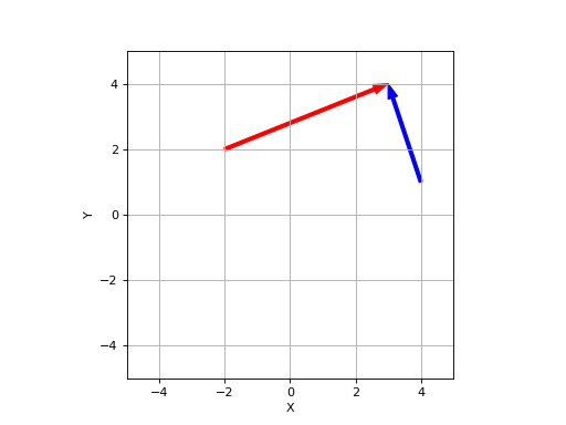

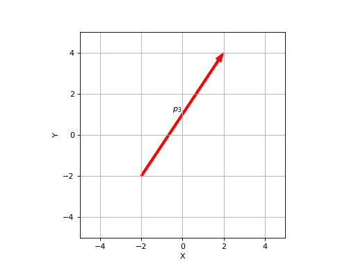
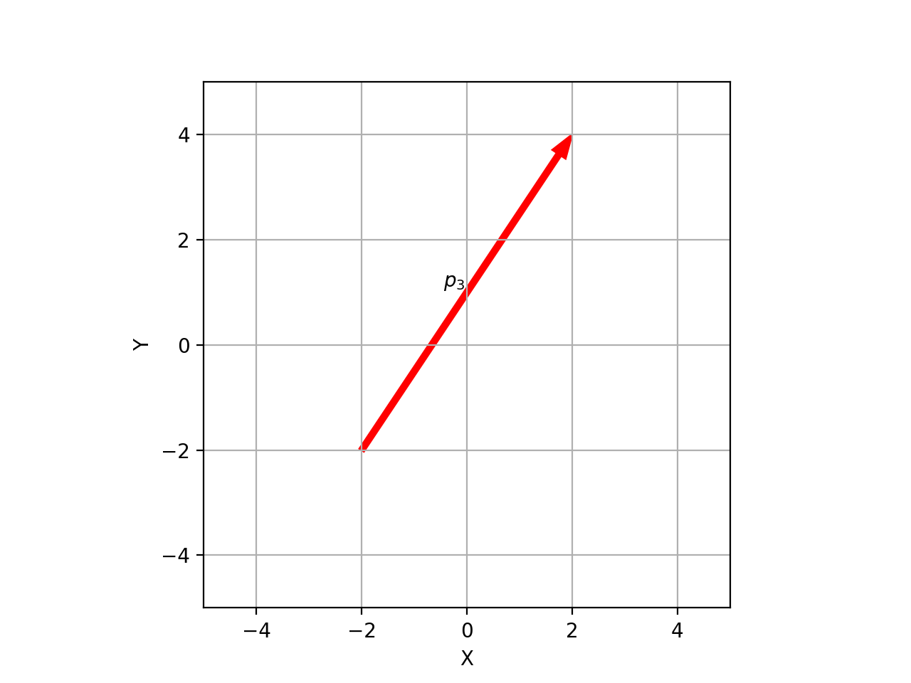
Example:

>>> from spatialmath.base import plotvol2, plot_arrow
>>> plotvol2(5)
>>> plot_arrow((-2, -2), (2, 4), label=r"$\mathit{p}_3$", color='r', width=0.1)

(Source code, png, hires.png, pdf)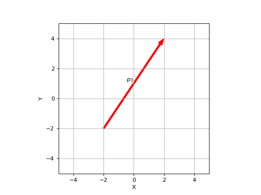

Seealso:

plot_homline()

plot_box(fmt=None, *, lbrt=None, lrbt=None, lbwh=None, bbox=None, ltrb=None, lb=None, lt=None, rb=None, rt=None, wh=None, centre=None, center=None, w=None, h=None, ax=None, filled=False, **kwargs)

Plot a 2D box using matplotlib

Parameters:

• lb (Union[List[float], Tuple[float, float], ndarray[Tuple[ResizeEventType[2]], dtype[floating]], None]) – left-bottom corner, defaults to None

• lt (Union[List[float], Tuple[float, float], ndarray[Tuple[ResizeEventType[2]], dtype[floating]], None]) – left-top corner, defaults to None

• rb (Union[List[float], Tuple[float, float], ndarray[Tuple[ResizeEventType[2]], dtype[floating]], None]) – right-bottom corner, defaults to None

• rt (Union[List[float], Tuple[float, float], ndarray[Tuple[ResizeEventType[2]], dtype[floating]], None]) – right-top corner, defaults to None

• wh (Union[List[float], Tuple[float, float], ndarray[Tuple[ResizeEventType[2]], dtype[floating]], None]) – width and height, if both are the same provide scalar, defaults to None

• centre (Union[List[float], Tuple[float, float], ndarray[Tuple[ResizeEventType[2]], dtype[floating]], None]) – centre of box, defaults to None (alias: center)

• w (Optional[float]) – width of box, defaults to None

• h (Optional[float]) – height of box, defaults to None

;param lbrt: left-bottom, right-top corners, defaults to None :type lbrt: array_like(4), optional :param lrbt: left-right, bottom-top corners, defaults to None :type lrbt: Union[List[float], Tuple[float, float, float, float], ndarray[Tuple[ResizeEventType[4]], dtype[floating]], None] :param lbwh: left-bottom corner, width and height, defaults to None :type lbwh: Union[List[float], Tuple[float, float, float, float], ndarray[Tuple[ResizeEventType[4]], dtype[floating]], None] :param ltrb: left-top, right-bottom corners, defaults to None :type ltrb: Union[List[float], Tuple[float, float, float, float], ndarray[Tuple[ResizeEventType[4]], dtype[floating]], None] :param ax: the axes to draw on, defaults to gca() :type ax: Optional[Axes] :param bbox: bounding box matrix, defaults to None :type bbox: Union[List[float], Tuple[float, float, float, float], ndarray[Tuple[ResizeEventType[4]], dtype[floating]], None] :param filled: fill the box, defaults to False (alias for Matplotlib fill) :type filled: bool :param thickness: line thickness (alias for Matplotlib linewidth) :type thickness: float, optional :type kwargs: :param kwargs: additional arguments passed to pyplot.Rectangle()

Returns:

the matplotlib object

Return type:

List[Artist]

Appearance is controlled by Matplotlib properties passed as keyword arguments, for example:

Parameters:

• color (array_like(3) or str) – box outline and fill color

• edgecolor (array_like(3) or str) – box outline colour (alias: ec)

• fillcolor (array_like(3) or str) – box fill colour

• filled (bool) – fill the box, defaults to False

• alpha (float, optional) – transparency, defaults to 1

• linestyle (str, optional) – box outline line style (alias: ls)

• linewidth (float, optional) – box outline line thickness (alias: lw)

Additionally, the line style and color can be conveniently set using the pyplot convention where the first argument is a fmt string, for example "r--" for dashed red. The allowable color letters are "rgbcmyk" and the line style characters are "-", "--", "-.", ":".

The box can be specified in many ways. Two corners:

• lb = left-bottom corner

• lt = left-top corner

• rb = right-bottom corner

• rt = right-top corner

Alternatively, one corner or centre plus the dimensons:

• wh = [width, height]

• w = width

• h = height

Alternatively, the box can be specified by a number of 4-vectors, various conventions are in use across different packages, so we support them all:

• lbrt = [umin, vmin, umax, vmax]

• lrbt = [umin, umax, vmin, vmax]

• lbwh = [umin, vmin, w, h]

• bbox same as lbwh

• ltrb = [umin, vmin, umax, vmax]`

For plots where the y-axis is inverted (eg. for images) then top is the smaller vertical coordinate (highest in the window).

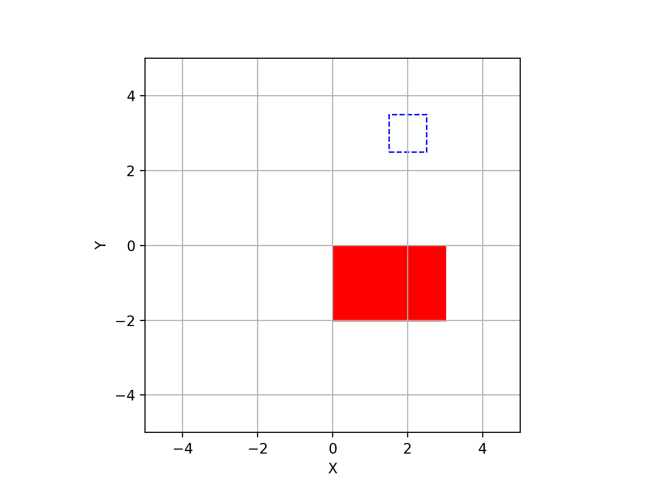
Example:

>>> plotvol2(5)
>>> plot_box("b--", centre=(2, 3), wh=1)  # w=h=1
>>> plot_box(lt=(0, 0), rb=(3, -2), filled=True, color="r")

(Source code, png, hires.png, pdf)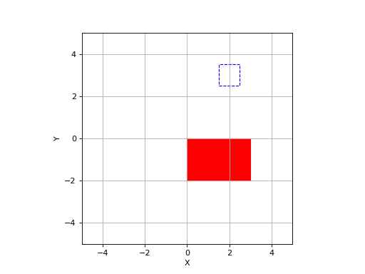

plot_circle(radius, centre, *fmt, resolution=50, ax=None, filled=False, **kwargs)

Plot a circle using matplotlib

Parameters:

• centre (Union[List[float], Tuple[float, float], ndarray[Tuple[ResizeEventType[2]], dtype[floating]]]) – centre of circle, defaults to (0,0)

• args

• radius (float) – radius of circle

• resolution (Optional[int]) – number of points on circumference, defaults to 50

Returns:

the matplotlib object

Return type:

List[Artist]

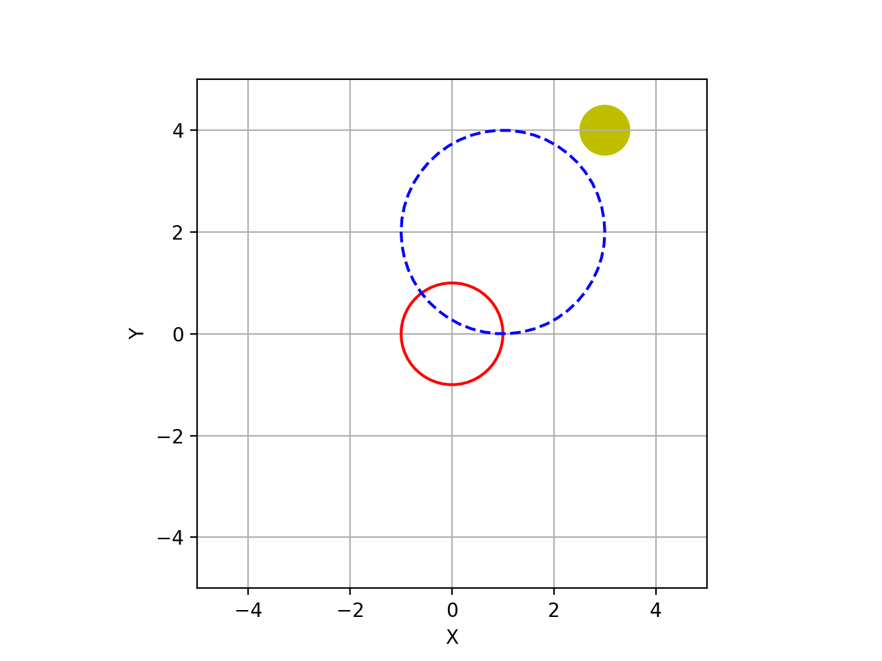
Plot or more circles. If centre is a 3xN array, then each column is taken as the centre of a circle. All circles have the same radius, color etc.

Example:

>>> from spatialmath.base import plotvol2, plot_circle
>>> plotvol2(5)
>>> plot_circle(1, (0,0), 'r')  # red circle
>>> plot_circle(2, (1, 2), 'b--')  # blue dashed circle
>>> plot_circle(0.5, (3,4), filled=True, facecolor='y')  # yellow filled circle

(Source code, png, hires.png, pdf)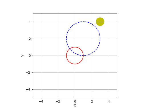

plot_ellipse(E, centre, *fmt, scale=1, confidence=None, resolution=40, inverted=False, ax=None, filled=False, **kwargs)

Plot an ellipse using matplotlib

Parameters:

• E (ndarray[Tuple[ResizeEventType[2], ResizeEventType[2]], dtype[floating]]) – matrix describing ellipse

• centre (Union[List[float], Tuple[float, float], ndarray[Tuple[ResizeEventType[2]], dtype[floating]]]) – centre of ellipse, defaults to (0, 0)

• scale (Optional[float]) – scale factor for the ellipse radii

• resolution (Optional[int]) – number of points on circumferece, defaults to 40

Returns:

the matplotlib object

Return type:

List[Artist]

The ellipse is defined by \(x^T \mat{E} x = s^2\) where \(x \in \mathbb{R}^2\) and \(s\) is the scale factor.

Note

For some common cases we require \(\mat{E}^{-1}\), for example:

• for robot manipulability \(\nu (\mat{J} \mat{J}^T)^{-1} \nu\) i

• a covariance matrix \((x - \mu)^T \mat{P}^{-1} (x - \mu)\) so to avoid inverting E twice to compute the ellipse, we flag that the inverse is provided using inverted.

Returns a set of resolution that lie on the circumference of a circle of given center and radius.

Example:

>>> from spatialmath.base import plotvol2, plot_ellipse
>>> plotvol2(5)
>>> plot_ellipse(np.array([[1, 1], [1, 2]]), [0,0], 'r')  # red ellipse
>>> plot_ellipse(np.array([[1, 1], [1, 2]]), [1, 2], 'b--')  # blue dashed ellipse
>>> plot_ellipse(np.array([[1, 1], [1, 2]]), [-2, -1], filled=True, facecolor='y')  # yellow filled ellipse

(Source code, png, hires.png, pdf)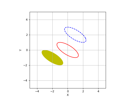

plot_homline(lines, *args, ax=None, xlim=None, ylim=None, **kwargs)

Plot homogeneous lines using matplotlib

Parameters:

• lines (Union[List[float], Tuple[float, float, float], ndarray[Tuple[ResizeEventType[3]], dtype[floating]], NDArray]) – homgeneous line or lines

• ax (Optional[Axes]) – axes to plot in, defaults to gca()

• kwargs – arguments passed to plot

Returns:

matplotlib object

Return type:

List[Artist]

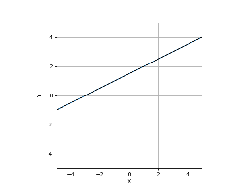
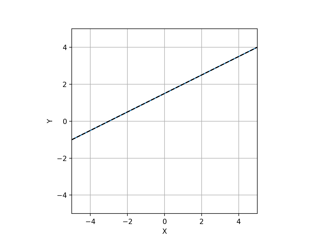
Draws the 2D line given in homogeneous form \(\ell[0] x + \ell[1] y + \ell[2] = 0\) in the current 2D axes.

If lines is a 3xN array then N lines are drawn, one per column.

Example:

>>> from spatialmath.base import plotvol2, plot_homline
>>> plotvol2(5)
>>> plot_homline((1, -2, 3))
>>> plot_homline((1, -2, 3), 'k--') # dashed black line

(Source code, png, hires.png, pdf)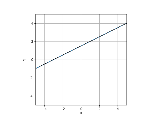

Seealso:

plot_arrow()

plot_point(pos, marker='bs', text=None, ax=None, textargs=None, textcolor=None, **kwargs)

Plot a point using matplotlib

Parameters:

• pos (Union[List[float], Tuple[float, float], ndarray[Tuple[ResizeEventType[2]], dtype[floating]]]) – position of marker

• marker (Optional[str]) – matplotlub marker style, defaults to ‘bs’

• text (Optional[str]) – text label, defaults to None

• ax (Optional[Axes]) – axes to plot in, defaults to gca()

Returns:

the matplotlib object

Return type:

List[Artist]

Plot one or more points, with optional text label.

• The color of the marker can be different to the color of the text, the marker color is specified by a single letter in the marker string.

• A point can have multiple markers, given as a list, which will be overlaid, for instance ["rx", "ro"] will give a ⨂ symbol.

• The optional text label is placed to the right of the marker, and vertically aligned.

• Multiple points can be marked if pos is a 2xn array or a list of coordinate pairs. In this case:

  • all points have the same text label

  • text can include the format string {} which is susbstituted for the point index, starting at zero

  • text can be a tuple containing a format string followed by vectors of shape(n). For example:

    ("#{0} a={1:.1f}, b={2:.1f}", a, b)
    

  will label each point with its index (argument 0) and consecutive elements of a and b which are arguments 1 and 2 respectively.

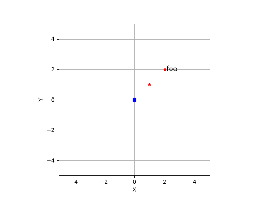
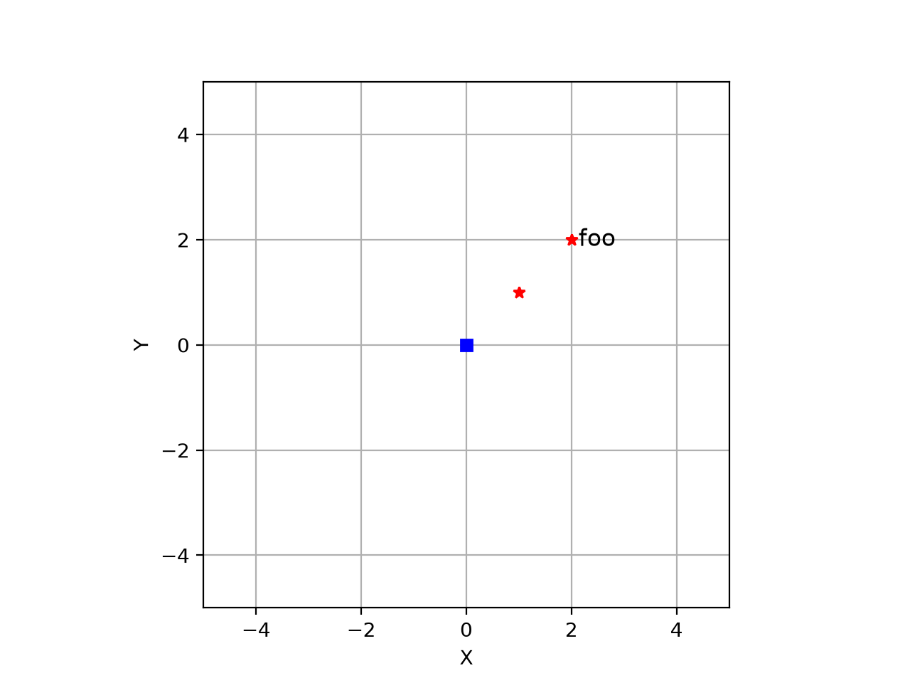
Example:

>>> from spatialmath.base import plotvol2, plot_point
>>> plotvol2(5)
>>> plot_point((0,0))        # plot default marker at coordinate (1,2)
>>> plot_point((1,1), 'r*')  # plot red star at coordinate (1,2)
>>> plot_point((2,2), 'r*', 'foo')  # plot red star at coordinate (1,2) and label it as 'foo'

(Source code, png, hires.png, pdf)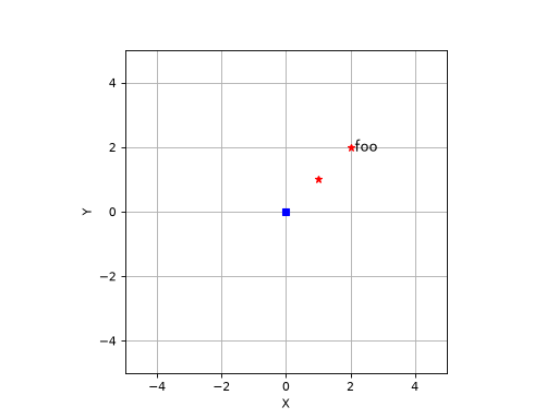

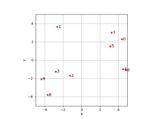
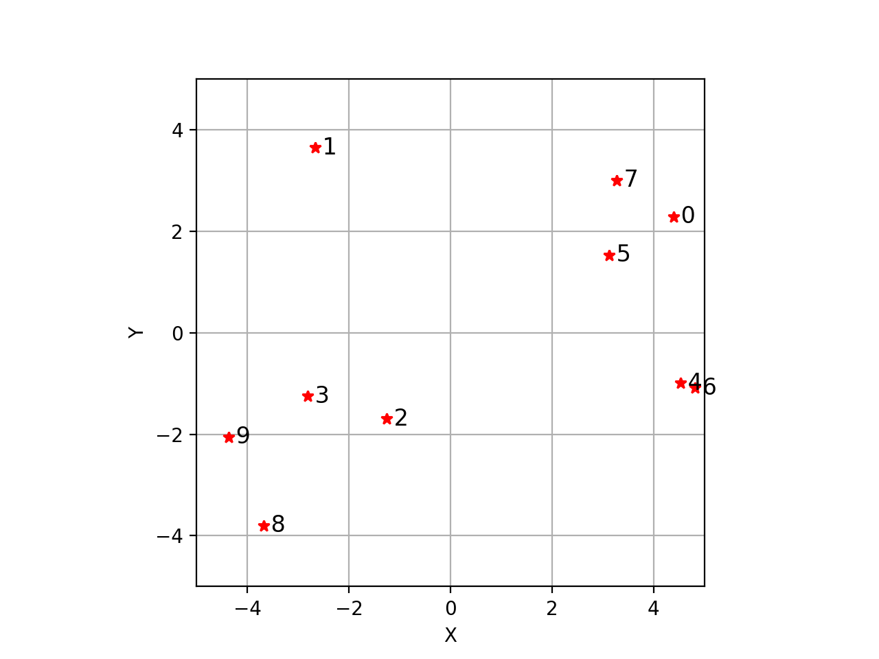
Plot red star at points defined by columns of p and label them sequentially from 0:

>>> p = np.random.uniform(size=(2,10), low=-5, high=5)
>>> plotvol2(5)
>>> plot_point(p, 'r*', '{0}')

(Source code, png, hires.png, pdf)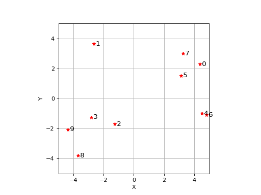

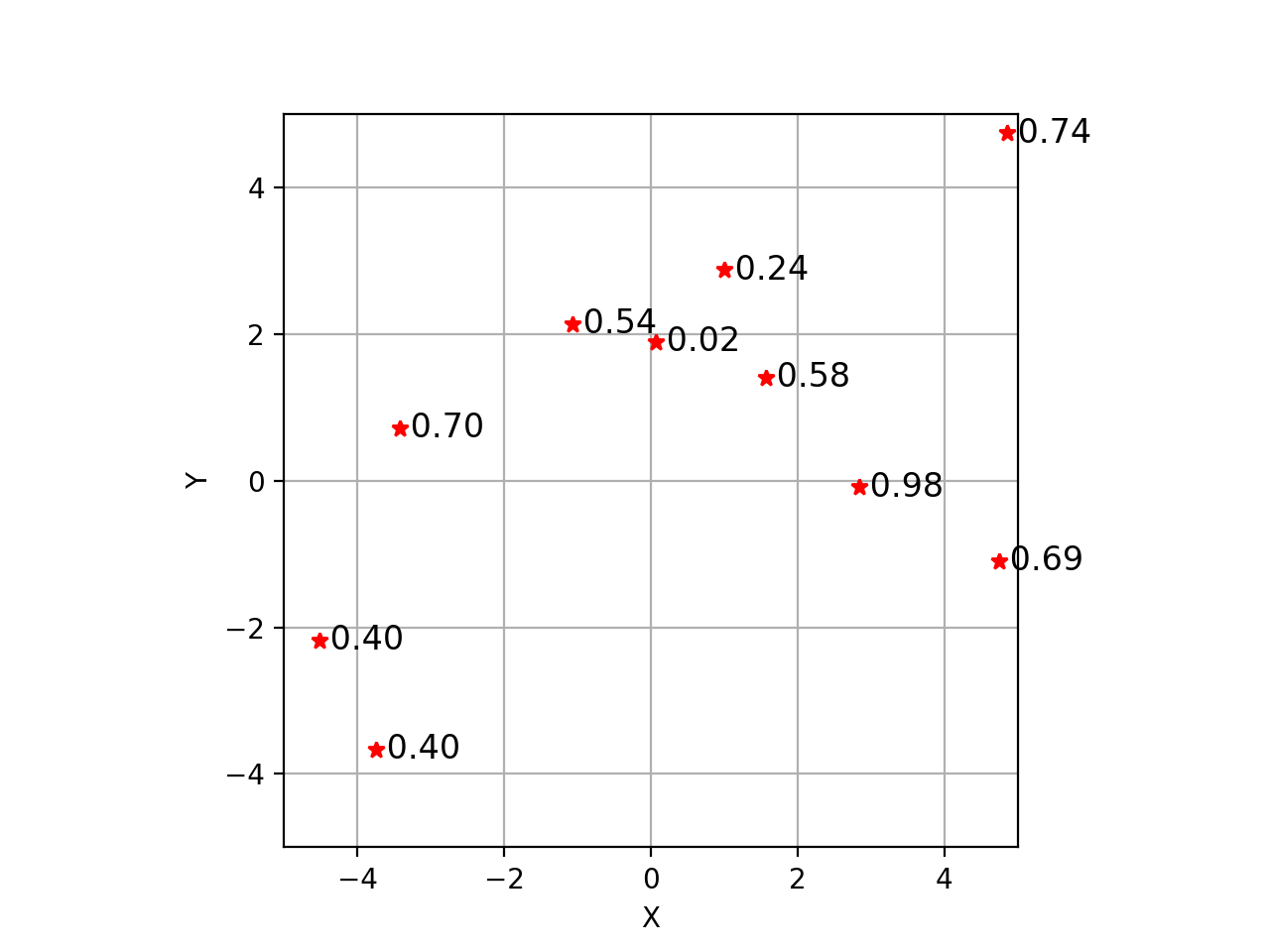
Plot red star at points defined by columns of p and label them all with successive elements of z

>>> p = np.random.uniform(size=(2,10), low=-5, high=5)
>>> value = np.random.uniform(size=(1,10))
>>> plotvol2(5)
>>> plot_point(p, 'r*', ('{1:.2f}', value))

(Source code, png, hires.png, pdf)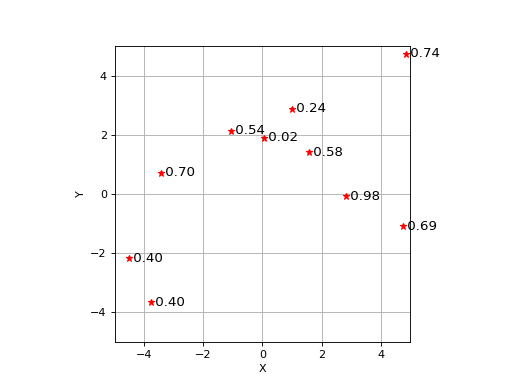

Seealso:

plot_text()

plot_polygon(vertices, *fmt, close=False, **kwargs)

Plot polygon

Parameters:

• vertices (NDArray) – vertices

• close (Optional[bool]) – close the polygon, defaults to False

• kwargs – arguments passed to Patch

Returns:

Matplotlib artist

Return type:

List[Artist]

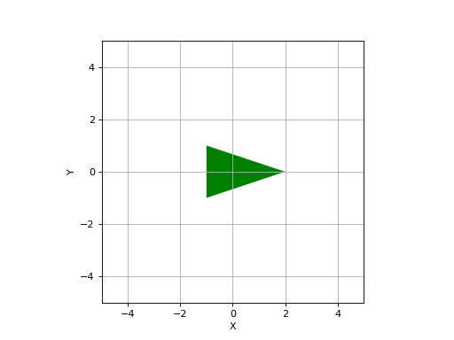
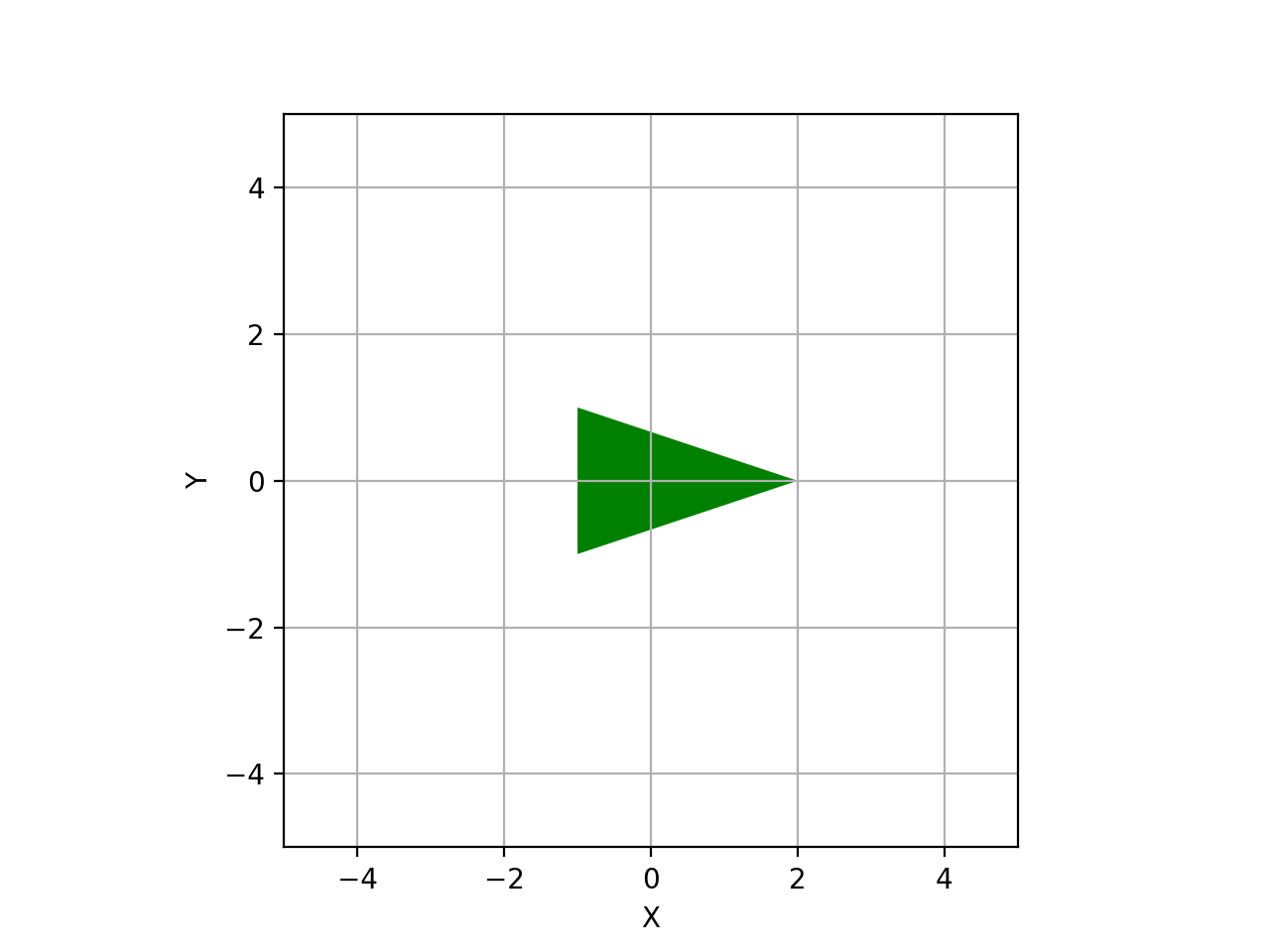
Example:

>>> from spatialmath.base import plotvol2, plot_polygon
>>> plotvol2(5)
>>> vertices = np.array([[-1, 2, -1], [1, 0, -1]])
>>> plot_polygon(vertices, filled=True, facecolor='g')  # green filled triangle

(Source code, png, hires.png, pdf)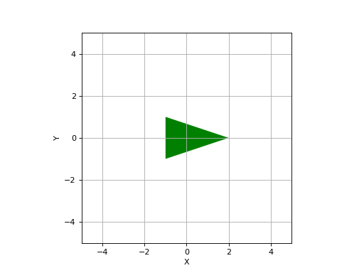

plot_text(pos, text, ax=None, color=None, **kwargs)

Plot text using matplotlib

Parameters:

• pos (Union[List[float], Tuple[float, float], ndarray[Tuple[ResizeEventType[2]], dtype[floating]]]) – position of text

• text (str) – text

• ax (Optional[Axes]) – axes to draw in, defaults to gca()

• color (Union[str, List[float], Tuple[float, float, float], ndarray[Tuple[ResizeEventType[3]], dtype[floating]], None]) – text color, defaults to None

• kwargs – additional arguments passed to pyplot.text()

Returns:

the matplotlib object

Return type:

List[Artist]

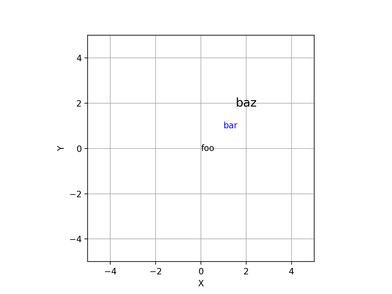
Example:

>>> from spatialmath.base import plotvol2, plot_text
>>> plotvol2(5)
>>> plot_text((1,3), 'foo')
>>> plot_text((2,2), 'bar', color='b')
>>> plot_text((2,2), 'baz', fontsize=14, horizontalalignment='centre')

(Source code, png, hires.png, pdf)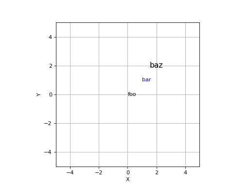

Seealso:

plot_point()

plotvol2(dim=None, ax=None, equal=True, grid=False, labels=True, new=False)

Create 2D plot area

Parameters:

• ax (Optional[Axes]) – axes of initializer, defaults to new subplot

• equal (Optional[bool]) – set aspect ratio to 1:1, default False

Returns:

initialized axes

Return type:

Axes

Initialize axes with dimensions given by dim which can be:

input	xrange	yrange
A (scalar)	-A:A	-A:A
[A, B]	A:B	A:B
[A, B, C, D]	A:B	C:D

Seealso:

plotvol3(), expand_dims()