Transforms in 3D

angvec2r(theta, v, unit='rad', tol=20)[source]

Create an SO(3) rotation matrix from rotation angle and axis

Parameters:

theta (float) – rotation
unit (str) – angular units: ‘rad’ [default], or ‘deg’
v (Union[List[float], Tuple[float, float, float], ndarray[Tuple[ResizeEventType[3]], dtype[floating]]]) – 3D rotation axis
tol (float) – Tolerance in units of eps for zero-rotation case, defaults to 20

Type:

float

Returns:

SO(3) rotation matrix

Return type:

SO3Array

Raises:

ValueError – bad arguments

angvec2r(θ, V) is an SO(3) orthonormal rotation matrix equivalent to a rotation of θ about the vector V.

>>> from spatialmath.base import angvec2r
>>> angvec2r(0.3, [1, 0, 0])  # rotx(0.3)
array([[ 1.        ,  0.        ,  0.        ],
       [ 0.        ,  0.95533649, -0.29552021],
       [ 0.        ,  0.29552021,  0.95533649]])
>>> angvec2r(0, [1, 0, 0])    # rotx(0)
array([[1., 0., 0.],
       [0., 1., 0.],
       [0., 0., 1.]])

Note

If θ == 0 then return identity matrix.
If θ ~= 0 then V must have a finite length.

Seealso:: angvec2tr() tr2angvec()
SymPy:: not supported

angvec2tr(theta, v, unit='rad')[source]

Create an SE(3) pure rotation from rotation angle and axis

Parameters:

theta (float) – rotation
unit (str) – angular units: ‘rad’ [default], or ‘deg’
v (Union[List[float], Tuple[float, float, float], ndarray[Tuple[ResizeEventType[3]], dtype[floating]]]) – 3D rotation axis

Returns:

SE(3) transformation matrix

Return type:

ndarray[Tuple[ResizeEventType[4], ResizeEventType[4]], dtype[floating]]

angvec2tr(θ, V) is an SE(3) homogeneous transformation matrix equivalent to a rotation of θ about the vector V.

>>> from spatialmath.base import angvec2tr
>>> angvec2tr(0.3, [1, 0, 0])  # rtotx(0.3)
array([[ 1.        ,  0.        ,  0.        ,  0.        ],
       [ 0.        ,  0.95533649, -0.29552021,  0.        ],
       [ 0.        ,  0.29552021,  0.95533649,  0.        ],
       [ 0.        ,  0.        ,  0.        ,  1.        ]])

Note

If θ == 0 then return identity matrix.
If θ ~= 0 then V must have a finite length.
The translational part is zero.

Seealso:: angvec2r() tr2angvec()
SymPy:: not supported

angvelxform(Γ, inverse=False, full=True, representation='rpy/xyz')[source]: DEPRECATED, use rotvelxform() instead

angvelxform_dot(Γ, Γd, full=True, representation='rpy/xyz')[source]: DEPRECATED, use rotvelxform() instead

delta2tr(d)[source]

Convert differential motion to SE(3)

Parameters:: Δ (array_like(6)) – differential motion as a 6-vector
Returns:: SE(3) matrix
Return type:: ndarray[Tuple[ResizeEventType[4], ResizeEventType[4]], dtype[floating]]

delta2tr(Δ) is an SE(3) matrix representing differential motion \(\Delta = [\delta_x, \delta_y, \delta_z, \theta_x, \theta_y, \theta_z]\).

>>> from spatialmath.base import delta2tr
>>> delta2tr([0.001, 0, 0, 0, 0.002, 0])
array([[ 1.   ,  0.   ,  0.002,  0.001],
       [ 0.   ,  1.   ,  0.   ,  0.   ],
       [-0.002,  0.   ,  1.   ,  0.   ],
       [ 0.   ,  0.   ,  0.   ,  1.   ]])

Reference:: Robotics, Vision & Control for Python, Section 3.1, P. Corke, Springer 2023.
Seealso:: tr2delta()
SymPy:: supported

eul2jac(angles)[source]

Euler angle rate Jacobian

Parameters:: angles (Union[List[float], Tuple[float, float, float], ndarray[Tuple[ResizeEventType[3]], dtype[floating]]]) – Euler angles (φ, θ, ψ)
Returns:: Jacobian matrix
Return type:: ndarray[Tuple[ResizeEventType[3], ResizeEventType[3]], dtype[floating]]

eul2jac(φ, θ, ψ) is a Jacobian matrix (3x3) that maps ZYZ Euler angle rates to angular velocity at the operating point specified by the Euler angles φ, ϴ, ψ.
eul2jac(𝚪) as above but the Euler angles are taken from 𝚪 which is a 3-vector with values (φ θ ψ).

Example:

>>> from spatialmath.base import eul2jac
>>> eul2jac([0.1, 0.2, 0.3])
array([[ 0.        , -0.09983342,  0.19767681],
       [ 0.        ,  0.99500417,  0.01983384],
       [ 1.        ,  0.        ,  0.98006658]])

Note

Used in the creation of an analytical Jacobian.
Angles in radians, rates in radians/sec.

Reference:: Robotics, Vision & Control for Python, Section 8.1.3, P. Corke, Springer 2023.
SymPy:: supported
Seealso:: angvelxform() rpy2jac() exp2jac()

eul2r(phi, theta=None, psi=None, unit='rad')[source]

Create an SO(3) rotation matrix from Euler angles

Parameters:

phi (Union[List[float], Tuple[float, float, float], ndarray[Tuple[ResizeEventType[3]], dtype[floating]], float]) – Z-axis rotation
theta (Optional[float]) – Y-axis rotation
psi (Optional[float]) – Z-axis rotation
unit (str) – angular units: ‘rad’ [default], or ‘deg’

Returns:

SO(3) rotation matrix

Return type:

SO3Array

R = eul2r(φ, θ, ψ) is an SO(3) orthonornal rotation matrix equivalent to the specified Euler angles. These correspond to rotations about the Z, Y, Z axes respectively.
R = eul2r(EUL) as above but the Euler angles are taken from EUL which is a 3-vector with values (φ θ ψ).

>>> from spatialmath.base import eul2r
>>> eul2r(0.1, 0.2, 0.3)
array([[ 0.902113  , -0.38355704,  0.19767681],
       [ 0.3875172 ,  0.92164909,  0.01983384],
       [-0.18979606,  0.0587108 ,  0.98006658]])
>>> eul2r([0.1, 0.2, 0.3])
array([[ 0.902113  , -0.38355704,  0.19767681],
       [ 0.3875172 ,  0.92164909,  0.01983384],
       [-0.18979606,  0.0587108 ,  0.98006658]])
>>> eul2r([10, 20, 30], unit='deg')
array([[ 0.71461018, -0.61309202,  0.33682409],
       [ 0.63371836,  0.77128058,  0.05939117],
       [-0.29619813,  0.17101007,  0.93969262]])

Seealso:: rpy2r() eul2tr() tr2eul()
SymPy:: supported

eul2tr(phi, theta=None, psi=None, unit='rad')[source]

Create an SE(3) pure rotation matrix from Euler angles

Parameters:

phi (float) – Z-axis rotation
theta (float) – Y-axis rotation
psi (float) – Z-axis rotation
unit (str) – angular units: ‘rad’ [default], or ‘deg’

Returns:

SE(3) transformation matrix

Return type:

ndarray[Tuple[ResizeEventType[4], ResizeEventType[4]], dtype[floating]]

R = eul2tr(PHI, θ, PSI) is an SE(3) homogeneous transformation matrix equivalent to the specified Euler angles. These correspond to rotations about the Z, Y, Z axes respectively.
R = eul2tr(EUL) as above but the Euler angles are taken from EUL which is a 3-vector with values (PHI θ PSI).

>>> from spatialmath.base import eul2tr
>>> eul2tr(0.1, 0.2, 0.3)
array([[ 0.902113  , -0.38355704,  0.19767681,  0.        ],
       [ 0.3875172 ,  0.92164909,  0.01983384,  0.        ],
       [-0.18979606,  0.0587108 ,  0.98006658,  0.        ],
       [ 0.        ,  0.        ,  0.        ,  1.        ]])
>>> eul2tr([0.1, 0.2, 0.3])
array([[ 0.902113  , -0.38355704,  0.19767681,  0.        ],
       [ 0.3875172 ,  0.92164909,  0.01983384,  0.        ],
       [-0.18979606,  0.0587108 ,  0.98006658,  0.        ],
       [ 0.        ,  0.        ,  0.        ,  1.        ]])
>>> eul2tr([10, 20, 30], unit='deg')
array([[ 0.71461018, -0.61309202,  0.33682409,  0.        ],
       [ 0.63371836,  0.77128058,  0.05939117,  0.        ],
       [-0.29619813,  0.17101007,  0.93969262,  0.        ],
       [ 0.        ,  0.        ,  0.        ,  1.        ]])

Note

By default, the translational component is zero but it can be set to a non-zero value.

Seealso:: rpy2tr() eul2r() tr2eul()
SymPy:: supported

exp2jac(v)[source]

Jacobian from exponential coordinate rates to angular velocity

Parameters:: v (ndarray[Tuple[ResizeEventType[3]], dtype[floating]]) – Exponential coordinates
Returns:: Jacobian matrix
Return type:: ndarray[Tuple[ResizeEventType[3], ResizeEventType[3]], dtype[floating]]

exp2jac(v) is a Jacobian matrix (3x3) that maps exponential coordinate rates to angular velocity at the operating point v.

>>> from spatialmath.base import exp2jac
>>> exp2jac([0.3, 0, 0])
array([[ 1.        ,  0.        ,  0.        ],
       [ 0.        ,  0.98506736, -0.14887837],
       [ 0.        ,  0.14887837,  0.98506736]])

Note

Used in the creation of an analytical Jacobian.

Reference:

- A compact formula for the derivative of a 3-D rotation in
  exponential coordinate
  Guillermo Gallego, Anthony Yezzi
  https://arxiv.org/pdf/1312.0788v1.pdf
- Robot Dynamics Lecture Notes
  Robotic Systems Lab, ETH Zurich, 2018
  https://ethz.ch/content/dam/ethz/special-interest/mavt/robotics-n-intelligent-systems/rsl-dam/documents/RobotDynamics2018/RD_HS2018script.pdf

SymPy:: supported
Seealso:: rotvelxform() eul2jac() rpy2jac()

exp2r(w)[source]

Create an SO(3) rotation matrix from exponential coordinates

Parameters:: w (Union[List[float], Tuple[float, float, float], ndarray[Tuple[ResizeEventType[3]], dtype[floating]]]) – exponential coordinate vector
Returns:: SO(3) rotation matrix
Return type:: ndarray[Tuple[ResizeEventType[4], ResizeEventType[4]], dtype[floating]]
Raises:: ValueError – bad arguments

exp2r(w) is an SO(3) orthonormal rotation matrix equivalent to a rotation of \(\| w \|\) about the vector \(\hat{w}\).

If w is zero then result is the identity matrix.

>>> from spatialmath.base import exp2r, rotx
>>> exp2r([0.3, 0, 0])
array([[ 1.        ,  0.        ,  0.        ],
       [ 0.        ,  0.95533649, -0.29552021],
       [ 0.        ,  0.29552021,  0.95533649]])
>>> rotx(0.3)
array([[ 1.        ,  0.        ,  0.        ],
       [ 0.        ,  0.95533649, -0.29552021],
       [ 0.        ,  0.29552021,  0.95533649]])

Note

Exponential coordinates are also known as an Euler vector

Seealso:: angvec2r() tr2angvec()
SymPy:: not supported

exp2tr(w)[source]

Create an SE(3) pure rotation matrix from exponential coordinates

Parameters:: w (Union[List[float], Tuple[float, float, float], ndarray[Tuple[ResizeEventType[3]], dtype[floating]]]) – exponential coordinate vector
Returns:: SO(3) rotation matrix
Return type:: ndarray[Tuple[ResizeEventType[4], ResizeEventType[4]], dtype[floating]]
Raises:: ValueError – bad arguments

exp2r(w) is an SO(3) orthonormal rotation matrix equivalent to a rotation of \(\| w \|\) about the vector \(\hat{w}\).

If w is zero then result is the identity matrix.

>>> from spatialmath.base import exp2tr, trotx
>>> exp2tr([0.3, 0, 0])
array([[ 1.        ,  0.        ,  0.        ,  0.        ],
       [ 0.        ,  0.95533649, -0.29552021,  0.        ],
       [ 0.        ,  0.29552021,  0.95533649,  0.        ],
       [ 0.        ,  0.        ,  0.        ,  1.        ]])
>>> trotx(0.3)
array([[ 1.        ,  0.        ,  0.        ,  0.        ],
       [ 0.        ,  0.95533649, -0.29552021,  0.        ],
       [ 0.        ,  0.29552021,  0.95533649,  0.        ],
       [ 0.        ,  0.        ,  0.        ,  1.        ]])

Note

Exponential coordinates are also known as an Euler vector

Seealso:: angvec2r() tr2angvec()
SymPy:: not supported

ishom(T, check=False, tol=20)[source]

Test if matrix belongs to SE(3)

Parameters:

T (Any) – SE(3) matrix to test
check (bool) – check validity of rotation submatrix
tol (float) – Tolerance in units of eps for rotation submatrix check, defaults to 20

Return type:

bool

Returns:

whether matrix is an SE(3) homogeneous transformation matrix

ishom(T) is True if the argument T is of dimension 4x4
ishom(T, check=True) as above, but also checks orthogonality of the rotation sub-matrix and validitity of the bottom row.

>>> from spatialmath.base import ishom
>>> import numpy as np
>>> T = np.array([[1, 0, 0, 3], [0, 1, 0, 4], [0, 0, 1, 5], [0, 0, 0, 1]])
>>> ishom(T)
True
>>> T = np.array([[1, 1, 0, 3], [0, 1, 0, 4], [0, 0, 1, 5], [0, 0, 0, 1]]) # invalid SE(3)
>>> ishom(T)  # a quick check says it is an SE(3)
True
>>> ishom(T, check=True) # but if we check more carefully...
False
>>> R = np.array([[1, 1, 0], [0, 1, 0], [0, 0, 1]])
>>> ishom(R)
False

Seealso:: isR() isrot() ishom2()

isrot(R, check=False, tol=20)[source]

Test if matrix belongs to SO(3)

Parameters:

R (Any) – SO(3) matrix to test
check (bool) – check validity of rotation submatrix
tol (float) – Tolerance in units of eps for rotation matrix test, defaults to 20

Return type:

bool

Returns:

whether matrix is an SO(3) rotation matrix

isrot(R) is True if the argument R is of dimension 3x3
isrot(R, check=True) as above, but also checks orthogonality of the rotation matrix.

>>> from spatialmath.base import isrot
>>> import numpy as np
>>> T = np.array([[1, 0, 0, 3], [0, 1, 0, 4], [0, 0, 1, 5], [0, 0, 0, 1]])
>>> isrot(T)
False
>>> R = np.array([[1, 0, 0], [0, 1, 0], [0, 0, 1]])
>>> isrot(R)
True
>>> R = R = np.array([[1, 1, 0], [0, 1, 0], [0, 0, 1]]) # invalid SO(3)
>>> isrot(R)  # a quick check says it is an SO(3)
True
>>> isrot(R, check=True) # but if we check more carefully...
False

Seealso:: isR() isrot2(), ishom()

oa2r(o, a)[source]

Create SO(3) rotation matrix from two vectors

Parameters:

o (array_like(3)) – 3D vector parallel to Y- axis
a (Union[List[float], Tuple[float, float, float], ndarray[Tuple[ResizeEventType[3]], dtype[floating]]]) – 3D vector parallel to the Z-axis

Returns:

SO(3) rotation matrix

Return type:

SO3Array

T = oa2tr(O, A) is an SO(3) orthonormal rotation matrix for a frame defined in terms of vectors parallel to its Y- and Z-axes with respect to a reference frame. In robotics these axes are respectively called the orientation and approach vectors defined such that R = [N O A] and N = O x A.

Steps:

N’ = O x A

O’ = A x N

normalize N’, O’, A

stack horizontally into rotation matrix

>>> from spatialmath.base import oa2r
>>> oa2r([0, 1, 0], [0, 0, -1])  # Y := Y, Z := -Z
array([[-1.,  0.,  0.],
       [ 0.,  1.,  0.],
       [ 0.,  0., -1.]])

Note

The A vector is the only guaranteed to have the same direction in the resulting rotation matrix
O and A do not have to be unit-length, they are normalized
O and A do not have to be orthogonal, so long as they are not parallel
The vectors O and A are parallel to the Y- and Z-axes of the equivalent coordinate frame.

Seealso:: oa2tr()
SymPy:: not supported

oa2tr(o, a)[source]

Create SE(3) pure rotation from two vectors

Parameters:

o (array_like(3)) – 3D vector parallel to Y- axis
a (Union[List[float], Tuple[float, float, float], ndarray[Tuple[ResizeEventType[3]], dtype[floating]]]) – 3D vector parallel to the Z-axis

Returns:

SE(3) transformation matrix

Return type:

ndarray[Tuple[ResizeEventType[4], ResizeEventType[4]], dtype[floating]]

T = oa2tr(O, A) is an SE(3) homogeneous transformation matrix for a frame defined in terms of vectors parallel to its Y- and Z-axes with respect to a reference frame. In robotics these axes are respectively called the orientation and approach vectors defined such that R = [N O A] and N = O x A.

Steps:

N’ = O x A

O’ = A x N

normalize N’, O’, A

stack horizontally into rotation matrix

>>> from spatialmath.base import oa2tr
>>> oa2tr([0, 1, 0], [0, 0, -1])  # Y := Y, Z := -Z
array([[-1.,  0.,  0.,  0.],
       [ 0.,  1.,  0.,  0.],
       [ 0.,  0., -1.,  0.],
       [ 0.,  0.,  0.,  1.]])

Seealso:: oa2r()
SymPy:: not supported

r2x(R, representation='rpy/xyz')[source]

Convert SO(3) matrix to angular representation

Parameters:

R (SO3Array) – SO(3) rotation matrix
representation (str) – rotational representation, defaults to “rpy/xyz”

Returns:

angular representation

Return type:

ndarray[Tuple[ResizeEventType[3]], dtype[floating]]

Convert an SO(3) rotation matrix to a minimal rotational representation \(\vec{\Gamma} \in \mathbb{R}^3\).

`representation`	Rotational representation
`"rpy/xyz"` `"arm"`	RPY angular rates in XYZ order (default)
`"rpy/zyx"` `"vehicle"`	RPY angular rates in XYZ order
`"rpy/yxz"` `"camera"`	RPY angular rates in YXZ order
`"eul"`	Euler angular rates in ZYZ order
`"exp"`	exponential coordinate rates

SymPy:: supported
Seealso:: x2r() tr2rpy() tr2eul() trlog()

rodrigues(w, theta=None)[source]

Rodrigues’ formula for 3D rotation

Parameters:

w (Union[List[float], Tuple[float, float, float], ndarray[Tuple[ResizeEventType[3]], dtype[floating]]]) – rotation vector
theta (Optional[float]) – rotation angle

Returns:

SO(3) matrix

Return type:

SO3Array

Compute Rodrigues’ formula for a rotation matrix given a rotation axis and angle.

\[\mat{R} = \mat{I}_{3 \times 3} + \sin \theta \skx{\hat{\vec{v}}} + (1 - \cos \theta) \skx{\hat{\vec{v}}}^2\]

>>> from spatialmath.base import *
>>> rodrigues([1, 0, 0], 0.3)
array([[ 1.        ,  0.        ,  0.        ],
       [ 0.        ,  0.95533649, -0.29552021],
       [ 0.        ,  0.29552021,  0.95533649]])
>>> rodrigues([0.3, 0, 0])
array([[ 1.        ,  0.        ,  0.        ],
       [ 0.        ,  0.95533649, -0.29552021],
       [ 0.        ,  0.29552021,  0.95533649]])

rot2jac(R, representation='rpy/xyz')[source]: DEPRECATED, use rotvelxform() instead

rotvelxform(Γ, inverse=False, full=False, representation='rpy/xyz')[source]

Rotational velocity transformation

Parameters:

𝚪 (array_like(3) or ndarray(3,3)) – angular representation or rotation matrix
representation (str, optional) – defaults to ‘rpy/xyz’
inverse (bool) – compute mapping from analytical rates to angular velocity
full (bool) – return 6x6 transform for spatial velocity

Returns:

rotation rate transformation matrix

Return type:

ndarray(3,3) or ndarray(6,6)

Computes the transformation from analytical rates \(\dvec{x}\) where the rotational part is expressed as the rate of change in some angular representation to spatial velocity \(\omega\), where rotation rate is expressed as angular velocity.

\[\vec{\omega} = \mat{A}(\Gamma) \dvec{x}\]

where \(\mat{A}\) is a 3x3 matrix and \(\Gamma \in \mathbb{R}^3\) is a minimal angular representation.

\(\mat{A}(\Gamma)\) is a function of the rotational representation which can be specified by the parameter 𝚪 as a 1D array, or by an SO(3) rotation matrix which will be converted to the representation.

`representation`	Rotational representation
`"rpy/xyz"` `"arm"`	RPY angular rates in XYZ order (default)
`"rpy/zyx"` `"vehicle"`	RPY angular rates in XYZ order
`"rpy/yxz"` `"camera"`	RPY angular rates in YXZ order
`"eul"`	Euler angular rates in ZYZ order
`"exp"`	exponential coordinate rates

If inverse==True return \(\mat{A}^{-1}\) computed using a closed-form solution rather than matrix inverse.

If full=True a block diagonal 6x6 matrix is returned which transforms analytic velocity to spatial velocity.

Note

Similar to eul2jac() rpy2jac() exp2jac() with full=False.

The analytical Jacobian is

\[\mat{J}_a(q) = \mat{A}^{-1}(\Gamma)\, \mat{J}(q)\]

where \(\mat{A}\) is computed with inverse==True and full=True.

Reference:

symbolic/angvelxform.ipynb in this Toolbox

Robot Dynamics Lecture Notes, Robotic Systems Lab, ETH Zurich, 2018 https://ethz.ch/content/dam/ethz/special-interest/mavt/robotics-n-intelligent-systems/rsl-dam/documents/RobotDynamics2018/RD_HS2018script.pdf

SymPy:: supported
Seealso:: rotvelxform_inv_dot() eul2jac() rpy2r() exp2jac()

rotvelxform_inv_dot(Γ, Γd, full=False, representation='rpy/xyz')[source]

Derivative of angular velocity transformation

Parameters:

𝚪 (array_like(3)) – angular representation
𝚪d (array_like(3)) – angular representation rate \(\dvec{\Gamma}\)
representation (str) – defaults to ‘rpy/xyz’
full (bool) – return 6x6 transform for spatial velocity

Returns:

derivative of inverse angular velocity transformation matrix

Return type:

Union[ndarray[Tuple[ResizeEventType[3], ResizeEventType[3]], dtype[floating]], ndarray[Tuple[ResizeEventType[6], ResizeEventType[6]], dtype[floating]]]

The angular rate transformation matrix \(\mat{A} \in \mathbb{R}^{6 \times 6}\) is such that

\[\dvec{x} = \mat{A}^{-1}(\Gamma) \vec{\nu}\]

where \(\dvec{x} \in \mathbb{R}^6\) is analytic velocity \((\vec{v}, \dvec{\Gamma})\), \(\vec{\nu} \in \mathbb{R}^6\) is spatial velocity \((\vec{v}, \vec{\omega})\), and \(\vec{\Gamma} \in \mathbb{R}^3\) is a minimal rotational representation.

The relationship between spatial and analytic acceleration is

\[\ddvec{x} = \dmat{A}^{-1}(\Gamma, \dot{\Gamma}) \vec{\nu} + \mat{A}^{-1}(\Gamma) \dvec{\nu}\]

and \(\dmat{A}^{-1}(\Gamma, \dot{\Gamma})\) is computed by this function.

`representation`	Rotational representation
`"rpy/xyz"` `"arm"`	RPY angular rates in XYZ order (default)
`"rpy/zyx"` `"vehicle"`	RPY angular rates in XYZ order
`"rpy/yxz"` `"camera"`	RPY angular rates in YXZ order
`"eul"`	Euler angular rates in ZYZ order
`"exp"`	exponential coordinate rates

If full=True a block diagonal 6x6 matrix is returned which transforms analytic analytic rotational acceleration to angular acceleration.

Reference:

symbolic/angvelxform.ipynb in this Toolbox

symbolic/angvelxform_dot.ipynb in this Toolbox

Seealso:: rotvelxform() eul2jac() rpy2r() exp2jac()

rotx(theta, unit='rad')[source]

Create SO(3) rotation about X-axis

Parameters:

theta (float) – rotation angle about X-axis
unit (str) – angular units: ‘rad’ [default], or ‘deg’

Returns:

SO(3) rotation matrix

Return type:

SO3Array

rotx(θ) is an SO(3) rotation matrix (3x3) representing a rotation of θ radians about the x-axis
rotx(θ, "deg") as above but θ is in degrees

>>> from spatialmath.base import rotx
>>> rotx(0.3)
array([[ 1.        ,  0.        ,  0.        ],
       [ 0.        ,  0.95533649, -0.29552021],
       [ 0.        ,  0.29552021,  0.95533649]])
>>> rotx(45, 'deg')
array([[ 1.        ,  0.        ,  0.        ],
       [ 0.        ,  0.70710678, -0.70710678],
       [ 0.        ,  0.70710678,  0.70710678]])

Seealso:: trotx()
SymPy:: supported

roty(theta, unit='rad')[source]

Create SO(3) rotation about Y-axis

Parameters:

theta (float) – rotation angle about Y-axis
unit (str) – angular units: ‘rad’ [default], or ‘deg’

Returns:

SO(3) rotation matrix

Return type:

SO3Array

roty(θ) is an SO(3) rotation matrix (3x3) representing a rotation of θ radians about the y-axis
roty(θ, "deg") as above but θ is in degrees

>>> from spatialmath.base import roty
>>> roty(0.3)
array([[ 0.95533649,  0.        ,  0.29552021],
       [ 0.        ,  1.        ,  0.        ],
       [-0.29552021,  0.        ,  0.95533649]])
>>> roty(45, 'deg')
array([[ 0.70710678,  0.        ,  0.70710678],
       [ 0.        ,  1.        ,  0.        ],
       [-0.70710678,  0.        ,  0.70710678]])

Seealso:: troty()
SymPy:: supported

rotz(theta, unit='rad')[source]

Create SO(3) rotation about Z-axis

Parameters:

theta (float) – rotation angle about Z-axis
unit (str) – angular units: ‘rad’ [default], or ‘deg’

Returns:

SO(3) rotation matrix

Return type:

SO3Array

rotz(θ) is an SO(3) rotation matrix (3x3) representing a rotation of θ radians about the z-axis
rotz(θ, "deg") as above but θ is in degrees

>>> from spatialmath.base import rotz
>>> rotz(0.3)
array([[ 0.95533649, -0.29552021,  0.        ],
       [ 0.29552021,  0.95533649,  0.        ],
       [ 0.        ,  0.        ,  1.        ]])
>>> rotz(45, 'deg')
array([[ 0.70710678, -0.70710678,  0.        ],
       [ 0.70710678,  0.70710678,  0.        ],
       [ 0.        ,  0.        ,  1.        ]])

Seealso:: trotz()
SymPy:: supported

rpy2jac(angles, order='zyx')[source]

Jacobian from RPY angle rates to angular velocity

Parameters:

angles (Union[List[float], Tuple[float, float, float], ndarray[Tuple[ResizeEventType[3]], dtype[floating]]]) – roll-pitch-yaw angles (⍺, β, γ)
order (str) – rotation order: ‘zyx’ [default], ‘xyz’, or ‘yxz’

Return type:

ndarray[Tuple[ResizeEventType[3], ResizeEventType[3]], dtype[floating]]

Returns:

Jacobian matrix

rpy2jac(⍺, β, γ) is a Jacobian matrix (3x3) that maps roll-pitch-yaw angle rates to angular velocity at the operating point (⍺, β, γ). These correspond to successive rotations about the axes specified by order:
- ‘zyx’ [default], rotate by γ about the z-axis, then by β about the new y-axis, then by ⍺ about the new x-axis. Convention for a mobile robot with x-axis forward and y-axis sideways.
- ‘xyz’, rotate by γ about the x-axis, then by β about the new y-axis, then by ⍺ about the new z-axis. Convention for a robot gripper with z-axis forward and y-axis between the gripper fingers.
- ‘yxz’, rotate by γ about the y-axis, then by β about the new x-axis, then by ⍺ about the new z-axis. Convention for a camera with z-axis parallel to the optic axis and x-axis parallel to the pixel rows.
rpy2jac(𝚪) as above but the roll, pitch, yaw angles are taken from 𝚪 which is a 3-vector with values (⍺, β, γ).

>>> from spatialmath.base import rpy2jac
>>> rpy2jac([0.1, 0.2, 0.3])
array([[ 0.93629336, -0.29552021,  0.        ],
       [ 0.28962948,  0.95533649,  0.        ],
       [-0.19866933,  0.        ,  1.        ]])

Note

Used in the creation of an analytical Jacobian.
Angles in radians, rates in radians/sec.

Reference:: Robotics, Vision & Control for Python, Section 8.1.3, P. Corke, Springer 2023.
SymPy:: supported
Seealso:: rotvelxform() eul2jac() exp2jac()

rpy2r(roll, pitch=None, yaw=None, *, unit='rad', order='zyx')[source]

Create an SO(3) rotation matrix from roll-pitch-yaw angles

Parameters:

roll (Union[List[float], Tuple[float, float, float], ndarray[Tuple[ResizeEventType[3]], dtype[floating]], float]) – roll angle
pitch (Optional[float]) – pitch angle
yaw (Optional[float]) – yaw angle
unit (str) – angular units: ‘rad’ [default], or ‘deg’
order (str) – rotation order: ‘zyx’ [default], ‘xyz’, or ‘yxz’

Returns:

SO(3) rotation matrix

Return type:

SO3Array

Raises:

ValueError – bad argument

rpy2r(⍺, β, γ) is an SO(3) orthonormal rotation matrix (3x3) equivalent to the specified roll (⍺), pitch (β), yaw (γ) angles angles. These correspond to successive rotations about the axes specified by order:
- ‘zyx’ [default], rotate by γ about the z-axis, then by β about the new y-axis, then by ⍺ about the new x-axis. Convention for a mobile robot with x-axis forward and y-axis sideways.
- ‘xyz’, rotate by γ about the x-axis, then by β about the new y-axis, then by ⍺ about the new z-axis. Convention for a robot gripper with z-axis forward and y-axis between the gripper fingers.
- ‘yxz’, rotate by γ about the y-axis, then by β about the new x-axis, then by ⍺ about the new z-axis. Convention for a camera with z-axis parallel to the optic axis and x-axis parallel to the pixel rows.
rpy2r(RPY) as above but the roll, pitch, yaw angles are taken from RPY which is a 3-vector with values (⍺, β, γ).

>>> from spatialmath.base import rpy2r
>>> rpy2r(0.1, 0.2, 0.3)
array([[ 0.93629336, -0.27509585,  0.21835066],
       [ 0.28962948,  0.95642509, -0.03695701],
       [-0.19866933,  0.0978434 ,  0.97517033]])
>>> rpy2r([0.1, 0.2, 0.3])
array([[ 0.93629336, -0.27509585,  0.21835066],
       [ 0.28962948,  0.95642509, -0.03695701],
       [-0.19866933,  0.0978434 ,  0.97517033]])
>>> rpy2r([10, 20, 30], unit='deg')
array([[ 0.81379768, -0.44096961,  0.37852231],
       [ 0.46984631,  0.88256412,  0.01802831],
       [-0.34202014,  0.16317591,  0.92541658]])

Seealso:: eul2r() rpy2tr() tr2rpy()

rpy2tr(roll, pitch=None, yaw=None, unit='rad', order='zyx')[source]

Create an SE(3) rotation matrix from roll-pitch-yaw angles

Parameters:

roll (float) – roll angle
pitch (float) – pitch angle
yaw (float) – yaw angle
unit (str) – angular units: ‘rad’ [default], or ‘deg’
order (str) – rotation order: ‘zyx’ [default], ‘xyz’, or ‘yxz’

Returns:

SE(3) transformation matrix

Return type:

ndarray[Tuple[ResizeEventType[4], ResizeEventType[4]], dtype[floating]]

rpy2tr(⍺, β, γ) is an SE(3) matrix (4x4) equivalent to the specified roll (⍺), pitch (β), yaw (γ) angles angles. These correspond to successive rotations about the axes specified by order:
- ‘zyx’ [default], rotate by γ about the z-axis, then by β about the new y-axis, then by ⍺ about the new x-axis. Convention for a mobile robot with x-axis forward and y-axis sideways.
- ‘xyz’, rotate by γ about the x-axis, then by β about the new y-axis, then by ⍺ about the new z-axis. Convention for a robot gripper with z-axis forward and y-axis between the gripper fingers.
- ‘yxz’, rotate by γ about the y-axis, then by β about the new x-axis, then by ⍺ about the new z-axis. Convention for a camera with z-axis parallel to the optic axis and x-axis parallel to the pixel rows.
rpy2tr(RPY) as above but the roll, pitch, yaw angles are taken from RPY which is a 3-vector with values (⍺, β, γ).

>>> from spatialmath.base import rpy2tr
>>> rpy2tr(0.1, 0.2, 0.3)
array([[ 0.93629336, -0.27509585,  0.21835066,  0.        ],
       [ 0.28962948,  0.95642509, -0.03695701,  0.        ],
       [-0.19866933,  0.0978434 ,  0.97517033,  0.        ],
       [ 0.        ,  0.        ,  0.        ,  1.        ]])
>>> rpy2tr([0.1, 0.2, 0.3])
array([[ 0.93629336, -0.27509585,  0.21835066,  0.        ],
       [ 0.28962948,  0.95642509, -0.03695701,  0.        ],
       [-0.19866933,  0.0978434 ,  0.97517033,  0.        ],
       [ 0.        ,  0.        ,  0.        ,  1.        ]])
>>> rpy2tr([10, 20, 30], unit='deg')
array([[ 0.81379768, -0.44096961,  0.37852231,  0.        ],
       [ 0.46984631,  0.88256412,  0.01802831,  0.        ],
       [-0.34202014,  0.16317591,  0.92541658,  0.        ],
       [ 0.        ,  0.        ,  0.        ,  1.        ]])

Note

By default, the translational component is zero but it can be set to a non-zero value.

Seealso:: eul2tr() rpy2r() tr2rpy()

tr2adjoint(T)[source]

Adjoint matrix

Parameters:: T (ndarray(4,4) or ndarray(3,3)) – SE(3) or SO(3) matrix
Returns:: adjoint matrix
Return type:: ndarray(6,6) or ndarray(3,3)

Computes an adjoint matrix that maps the Lie algebra between frames.

where \(\mat{T} \in \SE3\).

tr2jac(T) is an adjoint matrix (6x6) that maps spatial velocity or differential motion between frame {B} to frame {A} which are attached to the same moving body. The pose of {B} relative to {A} is represented by the homogeneous transform T = \({}^A {\bf T}_B\).

>>> from spatialmath.base import tr2adjoint, trotx
>>> T = trotx(0.3, t=[4,5,6])
>>> tr2adjoint(T)
array([[ 1.        ,  0.        ,  0.        ,  0.        , -4.2544179 ,
         6.54980369],
       [ 0.        ,  0.95533649, -0.29552021,  6.        , -1.18208083,
        -3.82134596],
       [ 0.        ,  0.29552021,  0.95533649, -5.        ,  3.82134596,
        -1.18208083],
       [ 0.        ,  0.        ,  0.        ,  1.        ,  0.        ,
         0.        ],
       [ 0.        ,  0.        ,  0.        ,  0.        ,  0.95533649,
        -0.29552021],
       [ 0.        ,  0.        ,  0.        ,  0.        ,  0.29552021,
         0.95533649]])

Reference:

Robotics, Vision & Control for Python, Section 3, P. Corke, Springer 2023.
Lie groups for 2D and 3D Transformations

SymPy:

supported

tr2angvec(T, unit='rad', check=False)[source]

Convert SO(3) or SE(3) to angle and rotation vector

Parameters:

R (ndarray(4,4) or ndarray(3,3)) – SE(3) or SO(3) matrix
unit (str) – ‘rad’ or ‘deg’
check (bool) – check that rotation matrix is valid

Returns:

\((\theta, {\bf v})\)

Return type:

Tuple[float, ndarray[Tuple[ResizeEventType[3]], dtype[floating]]]

Raises:

ValueError – bad arguments

(v, θ) = tr2angvec(R) is a rotation angle and a vector about which the rotation acts that corresponds to the rotation part of R.

By default the angle is in radians but can be changed setting unit=’deg’.

>>> from spatialmath.base import  troty, tr2angvec
>>> T = troty(45, 'deg')
>>> v, theta = tr2angvec(T)
>>> print(v, theta)
0.7853981633974483 [0. 1. 0.]

Note

If the input is SE(3) the translation component is ignored.

Seealso:: angvec2r() angvec2tr() tr2rpy() tr2eul()

tr2delta(T0, T1=None)[source]

Difference of SE(3) matrices as differential motion

Parameters:

T0 (ndarray[Tuple[ResizeEventType[4], ResizeEventType[4]], dtype[floating]]) – first SE(3) matrix
T1 (Optional[ndarray[Tuple[ResizeEventType[4], ResizeEventType[4]], dtype[floating]]]) – second SE(3) matrix

Returns:

Differential motion as a 6-vector

Return type:

ndarray[Tuple[ResizeEventType[6]], dtype[floating]]

Raises:

ValueError – bad arguments

tr2delta(T0, T1) is the differential motion Δ (6x1) corresponding to infinitessimal motion (in the T0 frame) from pose T0 to T1 which are SE(3) matrices.
tr2delta(T) as above but the motion is from the world frame to the pose represented by T.

The vector \(\Delta = [\delta_x, \delta_y, \delta_z, \theta_x, \theta_y, \theta_z]\) represents infinitessimal translation and rotation, and is an approximation to the instantaneous spatial velocity multiplied by time step.

>>> from spatialmath.base import tr2delta, trotx
>>> T1 = trotx(0.3, t=[4,5,6])
>>> T2 = trotx(0.31, t=[4,5.02,6])
>>> tr2delta(T1, T2)
array([ 0.        ,  0.01910673, -0.0059104 ,  0.00999983,  0.        ,
        0.        ])

Note

Δ is only an approximation to the motion T, and assumes that T0 ~ T1 or T ~ eye(4,4).
Can be considered as an approximation to the effect of spatial velocity over a a time interval, average spatial velocity multiplied by time.

Reference:: Robotics, Vision & Control for Python, Section 3.1, P. Corke, Springer 2023.
Seealso:: delta2tr()
SymPy:: supported

tr2eul(T, unit='rad', flip=False, check=False, tol=20)[source]

Convert SO(3) or SE(3) to ZYX Euler angles

Parameters:

R (ndarray(4,4) or ndarray(3,3)) – SE(3) or SO(3) matrix
unit (str) – ‘rad’ or ‘deg’
flip (bool) – choose first Euler angle to be in quadrant 2 or 3
check (bool) – check that rotation matrix is valid
tol (float) – Tolerance in units of eps for near-zero checks, defaults to 20

Type:

float

Returns:

ZYZ Euler angles

Return type:

ndarray[Tuple[ResizeEventType[3]], dtype[floating]]

tr2eul(R) are the Euler angles corresponding to the rotation part of R.

The 3 angles \([\phi, \theta, \psi]\) correspond to sequential rotations about the Z, Y and Z axes respectively.

By default the angles are in radians but can be changed setting unit=’deg’.

>>> from spatialmath.base import tr2eul, eul2tr
>>> T = eul2tr(0.2, 0.3, 0.5)
>>> print(T)
[[ 0.72642758 -0.62323169  0.28962948  0.        ]
 [ 0.63643066  0.76909626  0.0587108   0.        ]
 [-0.25934338  0.14167993  0.95533649  0.        ]
 [ 0.          0.          0.          1.        ]]
>>> tr2eul(T)
array([0.2, 0.3, 0.5])

Note

There is a singularity for the case where \(\theta=0\) in which case we arbitrarily set \(\phi = 0\) and \(\phi\) is set to \(\phi+\psi\).
If the input is SE(3) the translation component is ignored.

Seealso:: eul2r() eul2tr() tr2rpy() tr2angvec()
SymPy:: not supported

tr2jac(T)[source]

SE(3) Jacobian matrix

Parameters:: T (ndarray[Tuple[ResizeEventType[4], ResizeEventType[4]], dtype[floating]]) – SE(3) matrix
Returns:: Jacobian matrix
Return type:: ndarray[Tuple[ResizeEventType[6], ResizeEventType[6]], dtype[floating]]

Computes an Jacobian matrix that maps spatial velocity between two frames defined by an SE(3) matrix.

tr2jac(T) is a Jacobian matrix (6x6) that maps spatial velocity or differential motion from frame {B} to frame {A} where the pose of {B} elative to {A} is represented by the homogeneous transform T = \({}^A {\bf T}_B\).

>>> from spatialmath.base import tr2jac, trotx
>>> T = trotx(0.3, t=[4,5,6])
>>> tr2jac(T)
array([[ 1.        ,  0.        ,  0.        ,  0.        ,  0.        ,
         0.        ],
       [ 0.        ,  0.95533649, -0.29552021,  0.        ,  0.        ,
         0.        ],
       [ 0.        ,  0.29552021,  0.95533649,  0.        ,  0.        ,
         0.        ],
       [ 0.        ,  0.        ,  0.        ,  1.        ,  0.        ,
         0.        ],
       [ 0.        ,  0.        ,  0.        ,  0.        ,  0.95533649,
        -0.29552021],
       [ 0.        ,  0.        ,  0.        ,  0.        ,  0.29552021,
         0.95533649]])

Reference:: Robotics, Vision & Control for Python, Section 3.1, P. Corke, Springer 2023.
SymPy:: supported

tr2rpy(T, unit='rad', order='zyx', check=False, tol=20)[source]

Convert SO(3) or SE(3) to roll-pitch-yaw angles

Parameters:

R (ndarray(4,4) or ndarray(3,3)) – SE(3) or SO(3) matrix
unit (str) – ‘rad’ or ‘deg’
order (str) – ‘xyz’, ‘zyx’ or ‘yxz’ [default ‘zyx’]
check (bool) – check that rotation matrix is valid
tol (float) – Tolerance in units of eps, defaults to 20

Type:

float

Returns:

Roll-pitch-yaw angles

Return type:

ndarray[Tuple[ResizeEventType[3]], dtype[floating]]

Raises:

ValueError – bad arguments

tr2rpy(R) are the roll-pitch-yaw angles corresponding to the rotation part of R.

The 3 angles RPY = \([\theta_R, \theta_P, \theta_Y]\) correspond to sequential rotations about the Z, Y and X axes respectively. The axis order sequence can be changed by setting:

order='xyz' for sequential rotations about X, Y, Z axes
order='yxz' for sequential rotations about Y, X, Z axes

By default the angles are in radians but can be changed setting unit='deg'.

>>> from spatialmath.base import tr2rpy, rpy2tr
>>> T = rpy2tr(0.2, 0.3, 0.5)
>>> print(T)
[[ 0.83838664 -0.41834537  0.34942093  0.        ]
 [ 0.45801271  0.8882368  -0.03549297  0.        ]
 [-0.29552021  0.18979606  0.93629336  0.        ]
 [ 0.          0.          0.          1.        ]]
>>> tr2rpy(T)
array([0.2, 0.3, 0.5])

Note

There is a singularity for the case where \(\theta_P = \pi/2\) in which case we arbitrarily set \(\theta_R=0\) and \(\theta_Y = \theta_R + \theta_Y\).
If the input is SE(3) the translation component is ignored.

Seealso:: rpy2r() rpy2tr() tr2eul(), tr2angvec()
SymPy:: not supported

tr2str(T, orient='rpy/zyx', label='', fmt='{:.3g}', degsym=True, unit='deg')[source]

Convert SO(3) or SE(3) matrices to compact single-line string

Parameters:

T (Union[SO3Array, ndarray[Tuple[ResizeEventType[4], ResizeEventType[4]], dtype[floating]]]) – SE(3) or SO(3) matrix
label (str) – text label to put at start of line
orient (str) – 3-angle convention to use
fmt (str) – conversion format for each number in the format used with format
unit (str) – angular units: ‘rad’ [default], or ‘deg’

Returns:

formatted string

Return type:

str

Raises:

ValueError – bad argument

The matrix is formatted and returned as a string.

tr2str(R) converts the SO(3) rotation matrix to a compact single-line string:

[LABEL:] ORIENTATION UNIT

tr2str(T) prints the SE(3) homogoneous transform to a compact single-line string:

[LABEL:] [t=X, Y, Z;] ORIENTATION UNIT

Orientation is expressed in one of several formats:

‘rpy/zyx’ roll-pitch-yaw angles in ZYX axis order [default]

‘rpy/yxz’ roll-pitch-yaw angles in YXZ axis order

‘rpy/zyx’ roll-pitch-yaw angles in ZYX axis order

‘eul’ Euler angles in ZYZ axis order

‘angvec’ angle and axis
>>> from spatialmath.base import *
>>> T = transl(1,2,3) @ rpy2tr(10, 20, 30, 'deg')
>>> tr2str(T)
't = 1, 2, 3; rpy/zyx = 10°, 20°, 30°'
>>> tr2str(T, label='T', orient='angvec')
'T: t = 1, 2, 3; angvec = (35.8° | 0.124, 0.616, 0.778)'
>>> tr2str(T, label='T', orient='angvec', fmt='{:8.4g}')
'T: t =        1,        2,        3; angvec = (   35.82° |    0.124,   0.6156,   0.7782)'
Note

If the ‘rpy’ option is selected, then the particular angle sequence can be specified with the options ‘xyz’ or ‘yxz’ which are passed through to tr2rpy. ‘zyx’ is the default.

Default formatting is for compact display of data

For tabular data set fmt to a fixed width format such as fmt='{:.3g}'

Added in version 1.1.15:

seealso:: trprint() trprint2() tr2eul() tr2rpy() tr2angvec()
SymPy:: not supported

tr2x(T, representation='rpy/xyz')[source]

Convert SE(3) to an analytic representation

Parameters:

T (ndarray[Tuple[ResizeEventType[4], ResizeEventType[4]], dtype[floating]]) – pose as an SE(3) matrix
representation (str) – angular representation to use, defaults to “rpy/xyz”

Returns:

analytic vector representation

Return type:

ndarray[Tuple[ResizeEventType[6]], dtype[floating]]

Convert an SE(3) matrix into an equivalent vector representation \(\vec{x} = (\vec{t},\vec{r}) \in \mathbb{R}^6\) where rotation \(\vec{r} \in \mathbb{R}^3\) is encoded in a minimal representation.

`representation`	Rotational representation
`"rpy/xyz"` `"arm"`	RPY angular rates in XYZ order (default)
`"rpy/zyx"` `"vehicle"`	RPY angular rates in XYZ order
`"rpy/yxz"` `"camera"`	RPY angular rates in YXZ order
`"eul"`	Euler angular rates in ZYZ order
`"exp"`	exponential coordinate rates

SymPy:: supported
Seealso:: r2x()

tranimate(T, **kwargs)[source]

Animate a 3D coordinate frame

Parameters:

T (Union[SO3Array, ndarray[Tuple[ResizeEventType[4], ResizeEventType[4]], dtype[floating]]]) – SE(3) or SO(3) matrix
nframes (int) – number of steps in the animation [default 100]
repeat (bool) – animate in endless loop [default False]
interval (int) – number of milliseconds between frames [default 50]
wait (bool) – wait until animation is complete, default False
movie (str) – name of file to write MP4 movie into
kwargs (dict) – arguments passed to trplot

Return type:

str

tranimate(T) where T is an SO(3) or SE(3) matrix, animates a 3D coordinate frame moving from the world frame to the frame T in nsteps.
tranimate(I) where I is an iterable or generator, animates a 3D coordinate frame representing the pose of each element in the sequence of SO(3) or SE(3) matrices.

Examples:

>>> tranimate(transl(1,2,3)@trotx(1), frame='A', arrow=False, dim=[0, 5])
>>> tranimate(transl(1,2,3)@trotx(1), frame='A', arrow=False, dim=[0, 5], movie='spin.mp4')

Note

For Jupyter this works with the notebook and TkAgg backends.

Note

The animation occurs in the background after tranimate has returned. If block=True this blocks after the animation has completed.

Note

When saving animation to a file the animation does not appear on screen. A StopIteration exception may occur, this seems to be a matplotlib bug #19599

SymPy:: not supported
Seealso:: trplot, plotvol3

transl(x, y=None, z=None)[source]

Create SE(3) pure translation, or extract translation from SE(3) matrix

Create a translational SE(3) matrix

Parameters:

x (float) – translation along X-axis
y (float) – translation along Y-axis
z (float) – translation along Z-axis

Returns:

SE(3) transformation matrix

Return type:

numpy(4,4)

Raises:

ValueError – bad argument

T = transl( X, Y, Z ) is an SE(3) homogeneous transform (4x4) representing a pure translation of X, Y and Z.
T = transl( V ) as above but the translation is given by a 3-element list, dict, or a numpy array, row or column vector.

>>> from spatialmath.base import transl
>>> import numpy as np
>>> transl(3, 4, 5)
array([[1., 0., 0., 3.],
       [0., 1., 0., 4.],
       [0., 0., 1., 5.],
       [0., 0., 0., 1.]])
>>> transl([3, 4, 5])
array([[1., 0., 0., 3.],
       [0., 1., 0., 4.],
       [0., 0., 1., 5.],
       [0., 0., 0., 1.]])
>>> transl(np.array([3, 4, 5]))
array([[1., 0., 0., 3.],
       [0., 1., 0., 4.],
       [0., 0., 1., 5.],
       [0., 0., 0., 1.]])

Extract the translational part of an SE(3) matrix

Parameters:: x (numpy(4,4)) – SE(3) transformation matrix
Returns:: translation elements of SE(2) matrix
Return type:: ndarray(3)
Raises:: ValueError – bad argument

t = transl(T) is the translational part of a homogeneous transform T as a 3-element numpy array.

>>> from spatialmath.base import transl
>>> import numpy as np
>>> T = np.array([[1, 0, 0, 3], [0, 1, 0, 4], [0, 0, 1, 5], [0, 0, 0, 1]])
>>> transl(T)
array([3, 4, 5])

Note

This function is compatible with the MATLAB version of the Toolbox. It is unusual/weird in doing two completely different things inside the one function.

Seealso:: transl2()
SymPy:: supported

trexp(S, theta=None, check=True)[source]

Exponential of se(3) or so(3) matrix

Parameters:

S – se(3), so(3) matrix or equivalent twist vector
θ (float) – motion

Returns:

matrix exponential in SE(3) or SO(3)

Return type:

ndarray(4,4) or ndarray(3,3)

Raises:

ValueError – bad arguments

An efficient closed-form solution of the matrix exponential for arguments that are so(3) or se(3).

For so(3) the results is an SO(3) rotation matrix:

trexp(Ω) is the matrix exponential of the so(3) element Ω which is a 3x3 skew-symmetric matrix.
trexp(Ω, θ) as above but for an so(3) motion of Ωθ, where Ω is unit-norm skew-symmetric matrix representing a rotation axis and a rotation magnitude given by θ.
trexp(ω) is the matrix exponential of the so(3) element ω expressed as a 3-vector.
trexp(ω, θ) as above but for an so(3) motion of ωθ where ω is a unit-norm vector representing a rotation axis and a rotation magnitude given by θ. ω is expressed as a 3-vector.

>>> from spatialmath.base import trexp, skew
>>> trexp(skew([1, 2, 3]))
array([[-0.69492056,  0.71352099,  0.08929286],
       [-0.19200697, -0.30378504,  0.93319235],
       [ 0.69297817,  0.6313497 ,  0.34810748]])
>>> trexp(skew([1, 0, 0]), 2)  # revolute unit twist
array([[ 1.        ,  0.        ,  0.        ],
       [ 0.        , -0.41614684, -0.90929743],
       [ 0.        ,  0.90929743, -0.41614684]])
>>> trexp([1, 2, 3])
array([[-0.69492056,  0.71352099,  0.08929286],
       [-0.19200697, -0.30378504,  0.93319235],
       [ 0.69297817,  0.6313497 ,  0.34810748]])
>>> trexp([1, 0, 0], 2)  # revolute unit twist
array([[ 1.        ,  0.        ,  0.        ],
       [ 0.        , -0.41614684, -0.90929743],
       [ 0.        ,  0.90929743, -0.41614684]])

For se(3) the results is an SE(3) homogeneous transformation matrix:

trexp(Σ) is the matrix exponential of the se(3) element Σ which is a 4x4 augmented skew-symmetric matrix.
trexp(Σ, θ) as above but for an se(3) motion of Σθ, where Σ must represent a unit-twist, ie. the rotational component is a unit-norm skew-symmetric matrix.
trexp(S) is the matrix exponential of the se(3) element S represented as a 6-vector which can be considered a screw motion.
trexp(S, θ) as above but for an se(3) motion of Sθ, where S must represent a unit-twist, ie. the rotational component is a unit-norm skew-symmetric matrix.

>>> from spatialmath.base import trexp, skewa
>>> trexp(skewa([1, 2, 3, 4, 5, 6]))
array([[-0.42296095,  0.05284171,  0.90460588,  1.68665085],
       [ 0.88024744, -0.21301589,  0.42401495,  1.93258594],
       [ 0.2151011 ,  0.97561877,  0.04358362,  2.59841115],
       [ 0.        ,  0.        ,  0.        ,  1.        ]])
>>> trexp(skewa([1, 0, 0, 0, 0, 0]), 2)  # prismatic unit twist
array([[1., 0., 0., 2.],
       [0., 1., 0., 0.],
       [0., 0., 1., 0.],
       [0., 0., 0., 1.]])
>>> trexp([1, 2, 3, 4, 5, 6])
array([[-0.42296095,  0.05284171,  0.90460588,  1.68665085],
       [ 0.88024744, -0.21301589,  0.42401495,  1.93258594],
       [ 0.2151011 ,  0.97561877,  0.04358362,  2.59841115],
       [ 0.        ,  0.        ,  0.        ,  1.        ]])
>>> trexp([1, 0, 0, 0, 0, 0], 2)
array([[1., 0., 0., 2.],
       [0., 1., 0., 0.],
       [0., 0., 1., 0.],
       [0., 0., 0., 1.]])

Seealso:: trexp2()

trinterp(start, end, s, shortest=True)[source]

Interpolate SE(3) matrices

Parameters:

start (ndarray(4,4) or ndarray(3,3)) – initial SE(3) or SO(3) matrix value when s=0, if None then identity is used
end (ndarray(4,4) or ndarray(3,3)) – final SE(3) or SO(3) matrix, value when s=1
s (float) – interpolation coefficient, range 0 to 1
shortest (bool, default to True) – take the shortest path along the great circle for the rotation

Returns:

interpolated SE(3) or SO(3) matrix value

Return type:

ndarray(4,4) or ndarray(3,3)

Raises:

ValueError – bad arguments

trinterp(None, T, S) is a homogeneous transform (4x4) interpolated between identity when S=0 and T (4x4) when S=1.
trinterp(T0, T1, S) as above but interpolated between T0 (4x4) when S=0 and T1 (4x4) when S=1.
trinterp(None, R, S) is a rotation matrix (3x3) interpolated between identity when S=0 and R (3x3) when S=1.
trinterp(R0, R1, S) as above but interpolated between R0 (3x3) when S=0 and R1 (3x3) when S=1.

>>> from spatialmath.base import transl, trinterp
>>> T1 = transl(1, 2, 3)
>>> T2 = transl(4, 5, 6)
>>> trinterp(T1, T2, 0)
array([[1., 0., 0., 1.],
       [0., 1., 0., 2.],
       [0., 0., 1., 3.],
       [0., 0., 0., 1.]])
>>> trinterp(T1, T2, 1)
array([[1., 0., 0., 4.],
       [0., 1., 0., 5.],
       [0., 0., 1., 6.],
       [0., 0., 0., 1.]])
>>> trinterp(T1, T2, 0.5)
array([[1. , 0. , 0. , 2.5],
       [0. , 1. , 0. , 3.5],
       [0. , 0. , 1. , 4.5],
       [0. , 0. , 0. , 1. ]])
>>> trinterp(None, T2, 0)
array([[1., 0., 0., 0.],
       [0., 1., 0., 0.],
       [0., 0., 1., 0.],
       [0., 0., 0., 1.]])
>>> trinterp(None, T2, 1)
array([[1., 0., 0., 4.],
       [0., 1., 0., 5.],
       [0., 0., 1., 6.],
       [0., 0., 0., 1.]])
>>> trinterp(None, T2, 0.5)
array([[1. , 0. , 0. , 2. ],
       [0. , 1. , 0. , 2.5],
       [0. , 0. , 1. , 3. ],
       [0. , 0. , 0. , 1. ]])

Note

Rotation is interpolated using quaternion spherical linear interpolation (slerp).

Seealso:: spatialmath.base.quaternions.qlerp() trinterp2()

trinv(T)[source]

Invert an SE(3) matrix

Parameters:: T (ndarray[Tuple[ResizeEventType[4], ResizeEventType[4]], dtype[floating]]) – SE(3) matrix
Returns:: inverse of SE(3) matrix
Return type:: ndarray[Tuple[ResizeEventType[4], ResizeEventType[4]], dtype[floating]]
Raises:: ValueError – bad arguments

Computes an efficient inverse of an SE(3) matrix:

\(\begin{pmatrix} {\bf R} & t \\ 0\,0\,0 & 1 \end{pmatrix}^{-1} = \begin{pmatrix} {\bf R}^T & -{\bf R}^T t \\ 0\,0\, 0 & 1 \end{pmatrix}\)

>>> from spatialmath.base import trinv, trotx
>>> T = trotx(0.3, t=[4,5,6])
>>> trinv(T)
array([[ 1.        ,  0.        ,  0.        , -4.        ],
       [ 0.        ,  0.95533649,  0.29552021, -6.54980369],
       [ 0.        , -0.29552021,  0.95533649, -4.2544179 ],
       [ 0.        ,  0.        ,  0.        ,  1.        ]])
>>> T @ trinv(T)
array([[ 1.00000000e+00,  0.00000000e+00,  0.00000000e+00,
         0.00000000e+00],
       [ 0.00000000e+00,  1.00000000e+00, -9.37082533e-18,
         8.88178420e-16],
       [ 0.00000000e+00, -9.37082533e-18,  1.00000000e+00,
         0.00000000e+00],
       [ 0.00000000e+00,  0.00000000e+00,  0.00000000e+00,
         1.00000000e+00]])

SymPy:: supported

trlog(T, check=True, twist=False, tol=20)[source]

Logarithm of SO(3) or SE(3) matrix

Parameters:

R (ndarray(4,4) or ndarray(3,3)) – SE(3) or SO(3) matrix
check (bool) – check that matrix is valid
twist (bool) – return a twist vector instead of matrix [default]
tol (float) – Tolerance in units of eps for zero-rotation case, defaults to 20

Type:

float

Returns:

logarithm

Return type:

Union[ndarray[Tuple[ResizeEventType[3]], dtype[floating]], ndarray[Tuple[ResizeEventType[6]], dtype[floating]], ndarray[Tuple[ResizeEventType[4]], dtype[floating]]]

Raises:

ValueError – bad argument

An efficient closed-form solution of the matrix logarithm for arguments that are SO(3) or SE(3).

trlog(R) is the logarithm of the passed rotation matrix R which will be 3x3 skew-symmetric matrix. The equivalent vector from vex() is parallel to rotation axis and its norm is the amount of rotation about that axis.
trlog(T) is the logarithm of the passed homogeneous transformation matrix T which will be 4x4 augumented skew-symmetric matrix. The equivalent vector from vexa() is the twist vector (6x1) comprising [v w].

>>> from spatialmath.base import trlog, rotx, trotx
>>> trlog(trotx(0.3))
array([[ 0. ,  0. ,  0. ,  0. ],
       [ 0. ,  0. , -0.3,  0. ],
       [ 0. ,  0.3,  0. ,  0. ],
       [ 0. ,  0. ,  0. ,  0. ]])
>>> trlog(trotx(0.3), twist=True)
array([0. , 0. , 0. , 0.3, 0. , 0. ])
>>> trlog(rotx(0.3))
array([[ 0. ,  0. ,  0. ],
       [ 0. ,  0. , -0.3],
       [ 0. ,  0.3,  0. ]])
>>> trlog(rotx(0.3), twist=True)
array([0.3, 0. , 0. ])

Seealso:: trexp() vex() vexa()

trnorm(T)[source]

Normalize an SO(3) or SE(3) matrix

Parameters:: T (ndarray[Tuple[ResizeEventType[4], ResizeEventType[4]], dtype[floating]]) – SE(3) or SO(3) matrix
Returns:: normalized SE(3) or SO(3) matrix
Return type:: ndarray[Tuple[ResizeEventType[4], ResizeEventType[4]], dtype[floating]]
Raises:: ValueError – bad arguments

trnorm(R) is guaranteed to be a proper orthogonal matrix rotation matrix (3x3) which is close to the input matrix R (3x3).
trnorm(T) as above but the rotational submatrix of the homogeneous transformation T (4x4) is normalised while the translational part is unchanged.

The steps in normalization are:

If \(\mathbf{R} = [n, o, a]\)
Form unit vectors \(\hat{o}, \hat{a}\) from \(o, a\) respectively
Form the normal vector \(\hat{n} = \hat{o} \times \hat{a}\)
Recompute \(\hat{o} = \hat{a} \times \hat{n}\) to ensure that \(\hat{o}, \hat{a}\) are orthogonal
Form the normalized SO(3) matrix \(\mathbf{R} = [\hat{n}, \hat{o}, \hat{a}]\)

>>> from spatialmath.base import trnorm, troty
>>> from numpy import linalg
>>> T = troty(45, 'deg', t=[3, 4, 5])
>>> linalg.det(T[:3,:3]) - 1 # is a valid SO(3)
np.float64(0.0)
>>> T = T @ T @ T @ T @ T @ T @ T @ T @ T @ T @ T @ T @ T
>>> linalg.det(T[:3,:3]) - 1  # not quite a valid SE(3) anymore
np.float64(-3.3306690738754696e-16)
>>> T = trnorm(T)
>>> linalg.det(T[:3,:3]) - 1  # once more a valid SE(3)
np.float64(0.0)

Note

Only the direction of a-vector (the z-axis) is unchanged.
Used to prevent finite word length arithmetic causing transforms to become ‘unnormalized’, ie. determinant \(\ne 1\).

trotx(theta, unit='rad', t=None)[source]

Create SE(3) pure rotation about X-axis

Parameters:

theta (float) – rotation angle about X-axis
unit (str) – angular units: ‘rad’ [default], or ‘deg’
t (Union[List[float], Tuple[float, float, float], ndarray[Tuple[ResizeEventType[3]], dtype[floating]], None]) – 3D translation vector, defaults to [0,0,0]

Returns:

SE(3) transformation matrix

Return type:

ndarray[Tuple[ResizeEventType[4], ResizeEventType[4]], dtype[floating]]

trotx(θ) is a homogeneous transformation (4x4) representing a rotation of θ radians about the x-axis.
trotx(θ, 'deg') as above but θ is in degrees
trotx(θ, 'rad', t=[x,y,z]) as above with translation of [x,y,z]

>>> from spatialmath.base import trotx
>>> trotx(0.3)
array([[ 1.        ,  0.        ,  0.        ,  0.        ],
       [ 0.        ,  0.95533649, -0.29552021,  0.        ],
       [ 0.        ,  0.29552021,  0.95533649,  0.        ],
       [ 0.        ,  0.        ,  0.        ,  1.        ]])
>>> trotx(45, 'deg', t=[1,2,3])
array([[ 1.        ,  0.        ,  0.        ,  1.        ],
       [ 0.        ,  0.70710678, -0.70710678,  2.        ],
       [ 0.        ,  0.70710678,  0.70710678,  3.        ],
       [ 0.        ,  0.        ,  0.        ,  1.        ]])

Seealso:: rotx()
SymPy:: supported

troty(theta, unit='rad', t=None)[source]

Create SE(3) pure rotation about Y-axis

Parameters:

theta (float) – rotation angle about Y-axis
unit (str) – angular units: ‘rad’ [default], or ‘deg’
t (Union[List[float], Tuple[float, float, float], ndarray[Tuple[ResizeEventType[3]], dtype[floating]], None]) – 3D translation vector, defaults to [0,0,0]

Returns:

SE(3) transformation matrix

Return type:

ndarray[Tuple[ResizeEventType[4], ResizeEventType[4]], dtype[floating]]

troty(θ) is a homogeneous transformation (4x4) representing a rotation of θ radians about the y-axis.
troty(θ, 'deg') as above but θ is in degrees
troty(θ, 'rad', t=[x,y,z]) as above with translation of [x,y,z]

>>> from spatialmath.base import troty
>>> troty(0.3)
array([[ 0.95533649,  0.        ,  0.29552021,  0.        ],
       [ 0.        ,  1.        ,  0.        ,  0.        ],
       [-0.29552021,  0.        ,  0.95533649,  0.        ],
       [ 0.        ,  0.        ,  0.        ,  1.        ]])
>>> troty(45, 'deg', t=[1,2,3])
array([[ 0.70710678,  0.        ,  0.70710678,  1.        ],
       [ 0.        ,  1.        ,  0.        ,  2.        ],
       [-0.70710678,  0.        ,  0.70710678,  3.        ],
       [ 0.        ,  0.        ,  0.        ,  1.        ]])

Seealso:: roty()
SymPy:: supported

trotz(theta, unit='rad', t=None)[source]

Create SE(3) pure rotation about Z-axis

Parameters:

theta (float) – rotation angle about Z-axis
unit (str) – angular units: ‘rad’ [default], or ‘deg’
t (Union[List[float], Tuple[float, float, float], ndarray[Tuple[ResizeEventType[3]], dtype[floating]], None]) – 3D translation vector, defaults to [0,0,0]

Returns:

SE(3) transformation matrix

Return type:

ndarray[Tuple[ResizeEventType[4], ResizeEventType[4]], dtype[floating]]

trotz(θ) is a homogeneous transformation (4x4) representing a rotation of θ radians about the z-axis.
trotz(θ, 'deg') as above but θ is in degrees
trotz(θ, 'rad', t=[x,y,z]) as above with translation of [x,y,z]

>>> from spatialmath.base import trotz
>>> trotz(0.3)
array([[ 0.95533649, -0.29552021,  0.        ,  0.        ],
       [ 0.29552021,  0.95533649,  0.        ,  0.        ],
       [ 0.        ,  0.        ,  1.        ,  0.        ],
       [ 0.        ,  0.        ,  0.        ,  1.        ]])
>>> trotz(45, 'deg', t=[1,2,3])
array([[ 0.70710678, -0.70710678,  0.        ,  1.        ],
       [ 0.70710678,  0.70710678,  0.        ,  2.        ],
       [ 0.        ,  0.        ,  1.        ,  3.        ],
       [ 0.        ,  0.        ,  0.        ,  1.        ]])

Seealso:: rotz()
SymPy:: supported

trplot(T, style='arrow', color='blue', frame='', axislabel=True, axissubscript=True, textcolor='', labels=('X', 'Y', 'Z'), length=1, originsize=20, origincolor='', projection='ortho', block=None, anaglyph=None, wtl=0.2, width=None, ax=None, dims=None, d2=1.15, flo=(-0.05, -0.05, -0.05), **kwargs)[source]

Plot a 3D coordinate frame

Parameters:

T (Union[SO3Array, ndarray[Tuple[ResizeEventType[4], ResizeEventType[4]], dtype[floating]]]) – SE(3) or SO(3) matrix
style (str) – axis style: ‘arrow’ [default], ‘line’, ‘rgb’, ‘rviz’ (Rviz style)
color (Union[str, Tuple[str, str, str], List[str]]) – color of the lines defining the frame
textcolor (str) – color of text labels for the frame, default color
frame (str) – label the frame, name is shown below the frame and as subscripts on the frame axis labels
axislabel (bool) – display labels on axes, default True
axissubscript (bool) – display subscripts on axis labels, default True
labels (Tuple[str, str, str]) – labels for the axes, defaults to X, Y and Z
length (float) – length of coordinate frame axes, default 1
originsize (float) – size of dot to draw at the origin, 0 for no dot (default 20)
origincolor (str) – color of dot to draw at the origin, default is color
ax (Optional[Axes3D]) – the axes to plot into, defaults to current axes
block (Optional[bool]) – run the GUI main loop until all windows are closed, default True
dims (Union[List[float], Tuple[float, ...], ndarray[Any, dtype[floating]], None]) – dimension of plot volume as [xmin, xmax, ymin, ymax,zmin, zmax]. If dims is [min, max] those limits are applied to the x-, y- and z-axes.
anaglyph (Union[bool, str, Tuple[str, float], None]) – 3D anaglyph display, if True use use red-cyan glasses. To set the color pass a string like 'gb' for green-blue glasses. To set the disparity (default 0.1) provide second argument in a tuple, eg. ('rc', 0.2). Bigger disparity exagerates the 3D “pop out” effect.
wtl (float) – width-to-length ratio for arrows, default 0.2
projection (str) – 3D projection: ortho [default] or persp
width (Optional[float]) – width of lines, default 1
flo (Tuple[float, float, float]) – frame label offset, a vector for frame label text string relative to frame origin, default (-0.05, -0.05, -0.05)
d2 (float) – distance of frame axis label text from origin, default 1.15

Returns:

axes containing the frame

Return type:

Axes3DSubplot

Raises:

ValueError – bad arguments

Adds a 3D coordinate frame represented by the SO(3) or SE(3) matrix to the current axes. If T is iterable then multiple frames will be drawn.

The appearance of the coordinate frame depends on many parameters:

coordinate axes depend on:
- color of axes
- width of line
- length of line
- style which is one of:
  'arrow' [default], draw line with arrow head in color
  
  'line', draw line with no arrow head in color
  
  'rgb', frame axes are lines with no arrow head and red for X, green for Y, blue for Z; no origin dot
  
  'rviz', frame axes are thick lines with no arrow head and red for X, green for Y, blue for Z; no origin dot
coordinate axis labels depend on:
- axislabel if True [default] label the axis, default labels are X, Y, Z
- labels 3-list of alternative axis labels
- textcolor which defaults to color
- axissubscript if True [default] add the frame label frame as a subscript for each axis label
coordinate frame label depends on:
- frame the label placed inside {} near the origin of the frame
a dot at the origin
- originsize size of the dot, if zero no dot
- origincolor color of the dot, defaults to color

Examples:

trplot(T, frame='A')
trplot(T, frame='A', color='green')
trplot(T1, 'labels', 'UVW');

(Source code, png, hires.png, pdf)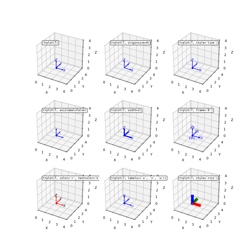

Note

If axes is specified the plot is drawn there, otherwise: - it will draw in the current figure (as given by gca()) - if no axes in the current figure, it will create a 3D axes - if no current figure, it will create one, and a 3D axes

Note

width can be set in the rgb or rviz styles to override the defaults which are 1 and 8 respectively.

Note

The anaglyph effect is induced by drawing two versions of the frame in different colors: one that corresponds to lens over the left eye and one to the lens over the right eye. The view for the right eye is from a view point shifted in the positive x-direction.

Note

The origin is normally indicated with a marker of the same color as the frame. The default size is 20. This can be disabled by setting its size to zero by originsize=0. For 'rgb' style the default is 0 but it can be set explicitly, and the color is as per the color option.

SymPy:: not supported
Seealso:: tranimate() plotvol3() axes_logic()

trprint(T, orient='rpy/zyx', label='', file=False, fmt='{:.3g}', degsym=True, unit='deg')[source]

Compact single-line display of SO(3) or SE(3) matrices

Parameters:

T (Union[SO3Array, ndarray[Tuple[ResizeEventType[4], ResizeEventType[4]], dtype[floating]]]) – SE(3) or SO(3) matrix :type T: ndarray(4,4) or ndarray(3,3)
label (str) – text label to put at start of line :type label: str
orient (str) – 3-angle convention to use :type orient: str
file (TextIO) – file to write formatted string to. [default, stdout] :type file: file object
fmt (str) – conversion format for each number in the format used with format :type fmt: str
unit (str) –
angular units: ‘rad’ [default], or ‘deg’ :type unit: str :return: formatted string :rtype: str :raises ValueError: bad argument

The matrix is formatted and written to file.

Return type:

str

trprint(R) prints the SO(3) rotation matrix to stdout in a compact single-line format:

[LABEL:] ORIENTATION UNIT

trprint(T) prints the SE(3) homogoneous transform to stdout in a compact single-line format:

[LABEL:] [t=X, Y, Z;] ORIENTATION UNIT

Orientation is expressed in one of several formats:

‘rpy/zyx’ roll-pitch-yaw angles in ZYX axis order [default]

‘rpy/yxz’ roll-pitch-yaw angles in YXZ axis order

‘rpy/zyx’ roll-pitch-yaw angles in ZYX axis order

‘eul’ Euler angles in ZYZ axis order

‘angvec’ angle and axis
>>> from spatialmath.base import *
>>> T = transl(1,2,3) @ rpy2tr(10, 20, 30, 'deg')
>>> trprint(T)
t = 1, 2, 3; rpy/zyx = 10°, 20°, 30°
't = 1, 2, 3; rpy/zyx = 10°, 20°, 30°'
>>> trprint(T, label='T', orient='angvec')
T: t = 1, 2, 3; angvec = (35.8° | 0.124, 0.616, 0.778)
'T: t = 1, 2, 3; angvec = (35.8° | 0.124, 0.616, 0.778)'
>>> trprint(T, label='T', orient='angvec', fmt='{:8.4g}')
T: t =        1,        2,        3; angvec = (   35.82° |    0.124,   0.6156,   0.7782)
'T: t =        1,        2,        3; angvec = (   35.82° |    0.124,   0.6156,   0.7782)'
Note

If the ‘rpy’ option is selected, then the particular angle sequence can be specified with the options ‘xyz’ or ‘yxz’ which are passed through to tr2rpy. ‘zyx’ is the default.

Default formatting is for compact display of data

For tabular data set fmt to a fixed width format such as fmt='{:.3g}'

Deprecated since version 1.1.15: file=None to get the string back without printing is deprecated - call tr2str() directly instead.

seealso:: tr2str() trprint2() tr2eul() tr2rpy() tr2angvec()
SymPy:: not supported

x2r(r, representation='rpy/xyz')[source]

Convert angular representation to SO(3) matrix

Parameters:

r (Union[List[float], Tuple[float, float, float], ndarray[Tuple[ResizeEventType[3]], dtype[floating]]]) – angular representation
representation (str) – rotational representation, defaults to “rpy/xyz”

Returns:

SO(3) rotation matrix

Return type:

SO3Array

Convert a minimal rotational representation \(\vec{\Gamma} \in \mathbb{R}^3\) to an SO(3) rotation matrix.

`representation`	Rotational representation
`"rpy/xyz"` `"arm"`	RPY angular rates in XYZ order (default)
`"rpy/zyx"` `"vehicle"`	RPY angular rates in XYZ order
`"rpy/yxz"` `"camera"`	RPY angular rates in YXZ order
`"eul"`	Euler angular rates in ZYZ order
`"exp"`	exponential coordinate rates

SymPy:: supported
Seealso:: r2x() rpy2r() eul2r() trexp()

x2tr(x, representation='rpy/xyz')[source]

Convert analytic representation to SE(3)

Parameters:

x (ndarray[Tuple[ResizeEventType[6]], dtype[floating]]) – analytic vector representation
representation (str, optional) – angular representation to use, defaults to “rpy/xyz”

Returns:

pose as an SE(3) matrix

Return type:

ndarray[Tuple[ResizeEventType[4], ResizeEventType[4]], dtype[floating]]

Convert a vector representation of pose \(\vec{x} = (\vec{t},\vec{r}) \in \mathbb{R}^6\) to SE(3), where rotation \(\vec{r} \in \mathbb{R}^3\) is encoded in a minimal representation to an equivalent SE(3) matrix.

`representation`	Rotational representation
`"rpy/xyz"` `"arm"`	RPY angular rates in XYZ order (default)
`"rpy/zyx"` `"vehicle"`	RPY angular rates in XYZ order
`"rpy/yxz"` `"camera"`	RPY angular rates in YXZ order
`"eul"`	Euler angular rates in ZYZ order
`"exp"`	exponential coordinate rates

SymPy:: supported
Seealso:: r2x()